...
Exercise 4: CDF, percentiles and probabilities
Recap
| Figure 1. The probability distribution function of the normal distribution or Gaussian distribution. The probabilities expressed as a percentage for various widths of standard deviations (σ) represent the area under the curve. |
|---|
Figure from Wikipedia. |

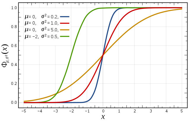
Figure 2. Cumulative distribution function for a normal |
|---|
Figure from Wikipedia. |
...
| borderColor | red |
|---|---|
| borderStyle | solid |
| title | Notes from Frederic 22/5/2018 |
...
Cumulative distribution function
The figures above illustrate the relationship between a normal distribution and its associated cumulative distribution function. The CDF is constructed from the area under the probability density function.
The CDF gives the probability that a value on the curve will be found to have a value less than or equal to the corresponding value on the x-axis. For example, in the figure, the probability for values less than or equal to X=0 is 50%.
The shape of the CDF curve is related to the shape of the normal distribution. The width of the CDF curve is directly related to the value of the standard deviation of the probability distribution function.
For an ensemble, the width is therefore related to the 'ensemble spread'. For a forecast ensemble where all values were the same, the CDF would be a vertical straight line.
Not all parameters will have a Gaussian distribution in values from the ensemble. This will be apparent in the exercises below.
Percentiles and probabilities
For a specified location, the CDF gives the probability that the parameter (for example, total precipitation) is below or equal to the percentile value, p, from the ensemble forecast. This means that the probability of the precipitation being above the value is 1-p.
A probability map then shows the spatial distribution of the precipitation exceeding a specific threshold, p, for example, a map showing the probability that the precipitation will exceed a threshold of 20mm in a 6hr period. A percentile map is very similar and shows the spatial distribution of the given percentile, for example, a map of total precipitation (in mm) for a percentile of 95%.
| Panel | ||||||
|---|---|---|---|---|---|---|
| ||||||
The idea of the exercise would be to show probabilities of precipitation by two different ways: 1 : CDF The exercise would be to plot the CDF at a specific location (maybe different forecast times), ask if the CDF caracterise a gaussian distribution (answer is not) and answer simple questions by reading the CDF : probability (1-p) that the precipitation exceeds 10mm, 20mm, 30mm, ... 2 : Probability map Probability map give a spatialized information of the precipitation exceeding a specific threshold (i.e. 1-p spatialized) but for just one p value. We can add a question where they set different thresholds and comment the probability maps over the Cevenes. |
Task 1: Plot the CDF for Toulouse
![]()
Enter the folder Probabilities in the openifs_2018 folder
Task 1: Cumulative distribution function
The figures above illustrate the relationship between a normal distribution and its associated cumulative distribution function. The CDF is constructed from the area under the probability density function.
The CDF gives the probability that a value on the curve will be found to have a value less than or equal to the corresponding value on the x-axis. For example, in the figure, the probability for values less than or equal to X=0 is 50%.
The shape of the CDF curve is related to the shape of the normal distribution. The width of the CDF curve is directly related to the value of the standard deviation of the probability distribution function.
For an ensemble, the width is therefore related to the 'ensemble spread'.
For a forecast ensemble where all values were the same, the CDF would be a vertical straight line.
Plot the CDFs
Enter the folder 'XXXXXXXXX'
| Warning |
|---|
TODO: update image |

![]()
This exercise uses the cdf.mv icon.
Right-click, select 'Edit' and then :
...
plot a CDF for Toulouse:
| Code Block | ||
|---|---|---|
| ||
param="tp"
station="TOU"
expID="ens_oper" |
Make sure useClusters='off'.
Do the same for the 2016 operational ensemble reforecast:
| Code Block |
|---|
expID="ens_2016" |
Compare the CDF from the different forecast ensembles.
| Panel | ||
|---|---|---|
| ||
Q. What can you say about the spread? Q. Why does the CDF not look like Figure 2 above? |
- Find a latitude/longitude point in the area of intense precipitation on 12Z 24/9/2012 and plot the CDF for MSLP (set station=[lat,lon] in the macro cdf.mv)
...
- )
...
| Warning |
|---|
TODO: can we get total precipitation (tp) for the CDF? |
Make sure useClusters='off'.
...
| borderColor | red |
|---|
...
Task 1. Plot percentiles of total precipitation
...