| Section |
|---|
| Column |
|---|
| 
|
| Column |
|---|
| | Panel |
|---|
Objectives
- Set-up a cylindrical projection over the United States.
- Apply land-shading on the coastlines.
- Load a grib file containing Mean-Sea level Presssure and visualise it using black isolines.
- Load a grib file containing Precipitation and visualise it using shading technique.
- Add a legend.
- Add a text.
- Draw the position of New-York City
- Draw a line to materialise the Xsection we are going to visualise in a next tutorial
You will need to download
|
|
|
...
| Section |
|---|
| Column |
|---|
| | Info |
|---|
|
subpage_lower_left_longitude | | subpage_lower_left_latitude | | subpage_upper_right_longitude | | subpage_upper_right_latitude |
|
| Code Block |
|---|
| theme | Confluence |
|---|
| language | python |
|---|
| title | Python - Setting a projection |
|---|
| collapse | true |
|---|
| from Magics.macro import *
#setting the output
output = output(
output_formats = ['png'],
output_name = "map_step1",
            output_name_first_page_number = "off"
        )
#settings of the geographical area
area = mmap(subpage_map_projection="cylindrical",
subpage_lower_left_longitude=-110.,
subpage_lower_left_latitude=20.,
subpage_upper_right_longitude=-30.,
subpage_upper_right_latitude=70.,
)
#Using a default coastlines to see the result
plot(output, area, mcoast()) |
|
| Column |
|---|
| 
|
|
...
| Section |
|---|
| Column |
|---|
| | Info |
|---|
| |
map_coastline_land_shade | | map_coastline_land_shade_colour | | map_coastline_colour | | map_grid_colour | | map_grid_line_style |
|
| Code Block |
|---|
| theme | Confluence |
|---|
| language | python |
|---|
| title | Python - Coastlines |
|---|
| collapse | true |
|---|
| from Magics.macro import *
#setting the output
output = output(
output_formats = ['png'],
output_name = "map_step2",
output_name_first_page_number = "off"
)
#settings of the geographical area
area = mmap(subpage_map_projection="cylindrical",
subpage_lower_left_longitude=-110.,
subpage_lower_left_latitude=20.,
subpage_upper_right_longitude=-30.,
subpage_upper_right_latitude=70.,
)
#settings of the caostlines
coast = mcoast(map_coastline_land_shade = "on",
map_coastline_land_shade_colour = "cream",
map_grid_line_style = "dash",
map_grid_colour = "grey",
map_label = "on",
map_coastline_colour = "grey")
plot(output, area, coast) |
|
| Column |
|---|
|  |
|
...
| Section |
|---|
| Column |
|---|
| | Info |
|---|
| |
mgrib action to load the data |
|---|
| grib_input_file_name |
| mcont action to define a contouring |
|---|
| contour_line_colour | | contour_line_thickness | | contour_highlight_colour | | contour_highlight_thickness | | contour_hilo | | contour_level_selection_type | | contour_interval | | legend | | contour_legend_text |
|
| Code Block |
|---|
| theme | Confluence |
|---|
| language | python |
|---|
| title | Python - CoastlinesMsl Visualisation |
|---|
| collapse | true |
|---|
| from Magics.macro import *
#setting the output
output = output(
output_formats = ['png'],
output_name = "map_step3",
output_name_first_page_number = "off"
)
#settings of the geographical area
area = mmap(subpage_map_projection="cylindrical",
subpage_lower_left_longitude=-110.,
subpage_lower_left_latitude=20.,
subpage_upper_right_longitude=-30.,
subpage_upper_right_latitude=70.,
)
#settings of the caostlines
coast = mcoast(map_coastline_land_shade = "on",
map_coastline_land_shade_colour = "cream",
map_grid_line_style = "dash",
map_grid_colour = "grey",
map_label = "on",
map_coastline_colour = "grey")
#Loading the msl Grib data
msl = mgrib(grib_input_file_name="msl.grib")
#Defining the controur
contour = mcont(contour_highlight_colour= "black",
contour_highlight_thickness= 4,
contour_hilo= "off",
contour_interval= 5.,
contour_label= "on",
contour_label_frequency= 2,
contour_label_height= 0.4,
contour_level_selection_type= "interval",
contour_line_colour= "black",
contour_line_thickness= 2,
legend='on',
contour_legend_text= "Mean Sea Level Pressure",
)
plot(output, area, coast, msl, contour) |
|
| Column |
|---|
|  |
|
...
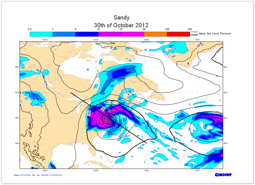
The goal of this exercise is to discover a bit more the diverse styles of visualisation offered by the mcont object.
Here we will work with shading, and we will use a different technique to setup the levels we want to contour.
| Section |
|---|
| Column |
|---|
| | Info |
|---|
|
mgrib action to load the data |
|---|
| grib_input_file_name | | grib_automatic_scaling | | grib_scaling_factor |
| mcont action to define a contouring |
|---|
| contour_line_colour | | contour_line_thickness | | contour_highlight_colour | | contour_highlight_thickness | | contour_hilo | | contour_level_selection_type | | contour_interval | | legend | | contour_legend_text |
|
| Code Block |
|---|
| theme | Confluence |
|---|
| language | python |
|---|
| title | Python - |
|---|
|
| Title| Use of Shading | | collapse | true |
|---|
| from Magics.macro import *
|
#settings of png
output_formats = ['png'],
|
coast output_name_first_page_number = "off"
)
|
##settingscoastlinesattributescoastmcoast(
mmap(subpage_map_projection="cylindrical",
        subpage_lower_left_longitude=-110.,
        subpage_lower_left_latitude=20.,
        subpage_upper_right_longitude=-30.,
        subpage_upper_right_latitude=70.,
    )
 #settings of the caostlines
coast = mcoast(map_coastline_land_shade = "on",
      map_coastline_land_shade_colour = "cream",
      map_grid_line_style = "dash",
map_grid_colour = " |
brown_colourbrown brown
##settings of the text (notice the Html formatting)
title = mtext(
text_lines = ["Hello World!", " <b>This is my first plot</b> !"],
text_font_size = "0.7",
text_colour = "charcoal"
)
#The plot command will now use the coast and title objects
plot(output, coast, title#Loading the msl Grib data
msl = mgrib(grib_input_file_name="msl.grib")
#Defining the controur
contour = mcont(contour_highlight_colour= "black",
contour_highlight_thickness= 4,
contour_hilo= "off",
contour_interval= 5.,
contour_label= "on",
contour_label_frequency= 2,
contour_label_height= 0.4,
contour_level_selection_type= "interval",
contour_line_colour= "black",
contour_line_thickness= 2,
legend='on',
contour_legend_text= "Mean Sea Level Pressure",
)
plot(output, area, coast, msl, contour) |
|
| Column |
|---|
| Image Added |
 Image Removed Image Removed |