...
In a sub-seasonal forecast, especially at the the longer ranges, the day-to-day variability of the river flow, with prediction of the actual expected flood severities, can not be expected due to the very high uncertainties. What is possible, is to rather give an indication of the river discharge anomalies and confidence in those predicted anomalies. As the forecast range increases, the uncertainty will also generally increase and with it the sharpness of the forecast will gradually decrease and more and more often the forecast is just going to show the climatologically expected conditions.
The determination generation of the sub-seasonal forecast signal is reflective of this and was designed to deliver a simple to understand categorical information on the anomalies and uncertainties present in the forecast, relative to the underlying climatology.
Climatological bins and anomaly categories
From the 660 reforecast values in the climate sample, 99 climate percentiles are determined (y-axis), which represent equally likely (1% chance) segments of the river discharge value range that occurred in the 20-year climatological sample. Figure 1 shows an example climate distribution, with only the deciles (every 10%), the two quartiles (25%, 50% and 75%), of which the middle (50%) is also called median, and few of the extreme percentiles are plotted near the minimum and maximum of the climatological range indicated by black crosses. Each of these percentiles have an equivalent river discharge value on the x-axis. From one percentile to the next, the river discharge value range is divided into 100 equally likely bins, some of which is indicated in Figure 1, such as bin1 of values below the 1st percentile, bin2 of values between the 1st and 2nd percentiles or bin 100 of river discharge values above the 99th percentiles, etc.
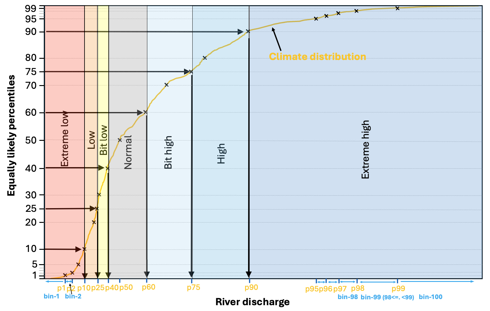
Figure 1. Schematic of the forecast anomaly categories, defined by the climatological distribution.
Based on the percentiles and the related 100 bins, there are seven anomaly categories defined. These are indicated in Figure 1 by shading. The two most extreme categories are the bottom and top 10% of the climatological distribution (<10% as red and 90%< as blue). Then the moderately low and high river discharge categories from 10-25% (orange) and 75-90% (middle-dark blue). The smallest negative and positive anomalies are defined by 25-40% and 60-75% and displayed by yellow and light blue colours in Figure 1. Finally, the normal condition category is defined from 40-60%, so the middle 1/5th of the distribution, coloured grey in Figure 1.
Forecast extremity rank computation
The forecast has 51 ensemble members, which all check where they fall in the 100 bins of the climate. This will be the anomaly or extremity value (called hereafter rank) of the ensemble members as one of the values from 1 to 100. For example, 1 will mean the forecast value is below the 1st climate percentile (i.e. extremely anomalously low), then 2 will mean the value is between the 1st and 2nd climate percentiles (i.e. slightly less extremely low), etc., and finally 100 will mean the forecast value is above the 99th climate percentile (i.e. extremely high as higher than 99% of all the considered reforecasts representing the model climate conditions for this time of year, location and lead time).
Figure 2 shows the process of determining the ranks for each ensemble member. The lowest member gets the rank of 54 (red r54 on the graph inFigure 2) by moving vertically until crossing the climatological distribution and then moving horizontally to the y-axis to determine the two bounding percentiles and thus the bin. In this case the lowest ensemble member value is between the 53rd and 54th percentile, which is bin54. Then all ensemble members similarly get a bin number, the 2nd lowest values with bin60 and so on until the largest ensemble member value getting bin 97 as a value between the 96th and 97th percentiles.

Figure 2. Schematic of the forecast extremity ranking of the 51 ensemble members and the 7 anomaly categories in the context of the climatological distribution.
Then the population and probabilities of each of the 7 anomaly categories are determined by counting the ensemble members in each category. In the example of Figure 2, there is no member in the 3 low flow anomaly categories, while the normal category has 2, the bit high category 13, the high category 17 and finally the extreme high category 18 ensemble members. These numbers then are converted to probabilities by dividing them with 51. The inset table in Figure 2 also shows the size (in probabilities) of the 7 categories. This highlights that the nomral category got, for example, 2 members, which results in 3.9% probability, but the expected climatological probability of this category is 20%.
Treatment of 0 values
The extremity rank can be computed for any value above 0 m3/s. However, the rank computation becomes undefined when the values drop to 0. This is actually a major problem, as large parts of the world has dry enough areas combined with small enough catchments to have near zero or totally 0 river discharge values. For this singularity case, a special treatment was defined. Here, all river discharge values below 0.1 m3/s are treated as 0, and will get the special rank computation. All the 0 ensemble member values get a randomly assigned rank from any of the percentiles that have 0 (i.e. below 0.1 m3/s) values in the model climatology. This effectively means, the 'rank-undefined' section of the ensemble forecast is going to be spread across the 'rank-undefined' section of the climatology during the rank computation.
Example-1:
Consider for example the following hypothetical example in Table 1. For simplicity, we represent the ensemble forecast by 21 members only (instead of 51). We also indicate below which values are considered as 0 (i.e. below 0.1 m3/s). In the 1st part of Table 1, you see the climatological percentile values, whether they are 0 or not, the possible rank values that can be assigned and the range for each of these rank values. Also, you see in the 2nd part in Table 1 the 21 ensemble member mean river discharge values, whether they are 0 or not, and then the assigned rank.
In this example, out of the 99 climate percentiles 58 are 0 (or considered 0), so this section is the undefined section where the rank computation is not directly possible. From the forecast, from the 21 represented ensemble members, 6 are (considered) 0. These 6 members will get ranks that come from the 1-58(/59) section of the 0 climatology, equally spanning it. For this example, the ranks would follow as 0, 58/5, 2*58/5, 3*58/5, 4*58/5 and finally 5*58/5, so 0, 11.6, 23.2, 34.8, 46.4 and 58. However, we can not assign fractional ranks, so we always choose the nearest integer number as rank. In this case, the ranks then would be for these 6 ensemble members: 0, 12, 23, 35, 46 and 58.
For the remaining ensemble members only few more are defined here, and the 61-96 percentiles and the related ranks are not listed here due to the limited space.
...
Table 1: Hypothetic example-1 of climate distribution and the related forecast ensemble distribution represented with only 21 members.
Example-2:
In this other super extreme example (Table 2) there is no measurable river discharge in the climatology at all. this, for example can happen somewhere in the middle of the desert in the Sahara, where basically all of the daily river discharge values in the longterm reanalysis are effectively 0, and thus all the 99 percentiles of the model climatology are 0.
In the forecast, however, there are few members which have noticeable discharge, so effectively are very extreme in the climatological context, even though the absolute values are not that large necessarily. So, out of the 21 members 17 are 0 (or considered 0), and those 17 members will get ranks assigned from the 0-section of the climatology, which is in this case all the way from 0 to 99. Thus, the ranks will be as follows: 0, 99/16 (so 6 as rounded value), 2*99/16 (12), 3*99/16 (19), ..., 15*99/16 (93) and 16*99/16 (99).
Moreover, all the forecast ensemble members, which are bigger than 0.1 m3/s, will get the rank of 99 for this case with the whole climatology being below 0.1 m3/s.
...
Table 2: Hypothetic example-2 of climate distribution and the related forecast ensemble distribution represented with only 21 members.
With this special treatment of the 0 singularity values, there is no need to mask areas on the new sub-seasonal and seasonal products. On the old version of the GloFAS seasonal forecasts, areas and time ranges, where the values were too small (effectively 0), were masked and the forecast values simply were not shown as 'undefined'.
For the new revised products, this special treatment will mean all of these 0 or near 0 cases will simply fall into an evenly distributed, very uncertain, on average near normal condition. Just as, following on from the 2nd example above, with no discharge in the climatology and no discharge in the forecast either, we will end up with a unified distribution of ranks from 0 to 99, evenly spanning the whole climatological range. Which means, if we average these ranks, we will get exactly the middle, the climate median, so no anomaly whatsoever.
This also means, for dry or very dry areas, there will never be a dry forecast anomaly, as that does not have any meaning (we can not go below 0), and therefore only neutral or positive anomalies are possible. The magnitude or severity of those positive anomalies then will be determined by the number and distribution of ensemble members being above the non-zero climate percentiles. If enough members will be above the non-zero climate percentiles and thus high enough fraction of the forecast will get high enough ranks, then on average the distribution of the 51 ensemble member ranks will show a pronounced enough shift from the neutral situation (i.e. when everything is 0 and the ranks are evenly distributed and the forecast end up looking totally normal).
...
weekly-mean-discharge-based climatology. The methodology to compute the anomaly and uncertainty information for the weekly mean sub-seasonal ensemble forecast is described here: