...
The revised sub-seasonal products cover calendar week periods (i.e. always Monday-Sunday), while the seasonal products are valid for whole calendar month periods as lead time. The forecast signal is derived from the relationship between the 'forecast-lead-time-averaged-river-discharge' (i.e. calendar week average or calendar month average) calendar weekly or monthly averaged river discharge and the climatological distribution of the same weekly- or monthly-mean averaged values. While this naturally works for the calendar months, the fixed calendar week lead times in the sub-seasonal will allow the users to directly compare forecasts from different forecast runs, as the verification period is fixed onto the calendar weeks. SoThis way, the evolution of the subsequent daily sub-seasonal forecast runs (always at 00 UTC) can be monitored by looking at the exact same verification period.
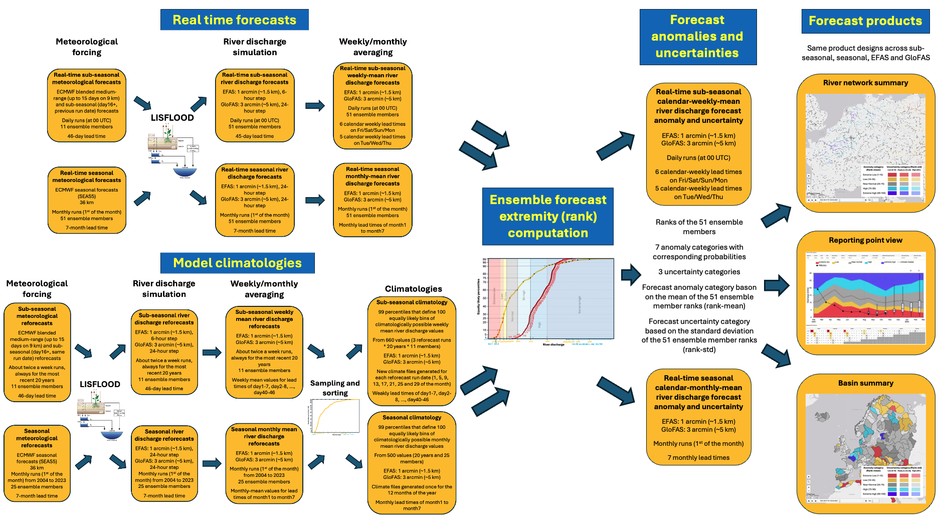
Figure 1. Flowchart of the sub-seasonal and seasonal anomaly and uncertainty information generaiton signal generation methodology.
...
The generation of the sub-seasonal and seasonal forecast signal relies on few major steps. The process is illustrated by a flowchart in Figure 1. The first ingredient is the actual forecast that is produced in real time.
Real time forecasts
This part is the hydrological forecasts produced in real time. This will give the actual predicted conditions for the sub-seasonal products that will be compared to the climatologies to derive the forecast anomaly and uncertainty. In the following, we describe the characteristics of these real time forecast simulations. Where appropriate, the difference between EFAS and GloFAS is specified. If there is no EFAS/GloFAS mentioned, then the method is identical between the two forecast systems:
...