Since the implementation of EFAS version 5.4 and GloFAS v4.3 in 2025, the same design of products are used for both the sub-seasonal and seasonal range forecasts in EFAS and GloFAS. This means, the previous EFAS/GloFAS seasonal products and the EFAS sub-seasonal product were replaced by the new ones, while for GloFAS the sub-seasonal product was newly introduced.
The generation of the sub-seasonal and seasonal forecast signal relies on few major steps. The process is illustrated by a flowchart in Figure 1.
The revised sub-seasonal products cover calendar week periods (i.e. always Monday-Sunday), while the seasonal products are valid for whole calendar month periods. The forecast signal is derived from the relationship between the calendar weekly or monthly averaged river discharge and the climatological distribution of the same weekly- or monthly-averaged values. While this naturally works for the calendar months, the fixed calendar week lead times in the sub-seasonal allow the users to directly compare forecasts from different forecast runs, as the verification period is fixed onto the calendar weeks. This way, the evolution of the subsequent daily sub-seasonal forecast runs (always at 00 UTC) can be monitored by looking at the exact same verification period.
The forecast anomaly and uncertainty signal is derived by comparing the real time forecast (top left section in Figure 1) to the 99-value model climate percentiles. The climatology is generated using reforecast over a 20-year period, which provides range-dependent climate percentiles that change with the lead time. The climate generation is described in Figure 1 in the bottom right corner.
The following step in generating anomaly and uncertainty signals is to determine, how extreme the ensemble members of the forecast are in the context of the climatological behaviour, which is represented by the 99 percentiles and the corresponding 100 equally likely bins of the climate range. This is done by ranking each ensemble member and sorting them into one of the 100 climatological bins. This gives 51 ranks, that range from 1 to 100.
In order to display the information of the 51 ensemble values, which all have either the calendar-weekly- or calendar-monthly-mean river discharge values or the 51 climatological ranks, a simplification was necessary. For this, 7 anomaly categories were defined from
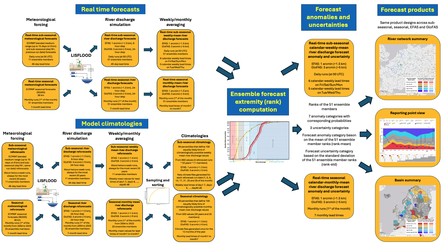
Figure 1. Flowchart of the sub-seasonal and seasonal anomaly and uncertainty signal generation methodology.
...
- Hydrological model used: LISFLOOD (LINK!)
- Meteorological forcing:
- Sub-seasonal:
- The combination of the 9km (horizontal resolution) ECMWF ensemble forecasts (LINK!) and the 36km ECMWF sub-seasonal forecasts (LINK!) from the same run date
- The low-resolution sub-seasonal and high-resolution medium-range forcings are taken from the same forecast run date. The timing of the availability of the low-resolution forecasts is not an issue here, as these reforecasts are only produced retrospectively without any time constraint.
- The high- and low-resolution forcing is currently combined by a simple mechanical blending by using the high resolution meteorological forcing for days 1-15, while the low-resolution meteorological forcing for days 16-46, for each of the 11 ensemble members.
- The blending can create inconsistencies locally over very complex orographical areas, due to the resolution change at day15, and also there could be some smaller inconsistencies between the ensemble because of the forcing change from 15 to 16 day, due to the mechanical blending which will mix different weather conditions from the low- and high-resolution meteorological data. However, overall as an ensemble of 11 scenarios, this will not be expected to lead to any larger discontinuities.
- Seasonal:
- 36 km seasonal forecasts (SEAS5, LINK)
- Number of ensemble members:
- Sub-seasonal has 11 ensemble members (one unperturbed and 10 perturbed) to represent the equally likely forecast scenarios of the future.
- Seasonal has 25 ensemble members (one unperturbed and 10 perturbed) to represent the equally likely forecast scenarios of the future.
- Sub-seasonal:
- River resolution:
- 1 arcmin (~1.5 km) in EFAS
- 3 arcmin (~5 km) in GloFAS.
- Run frequency:
- Sub-seasonal reforecasts are generated always for the past 20 years. Before 12 Nov 2024, they were generated twice-weekly on Mondays and Thursdays (at 00 UTC), while from 12 Nov 2024 they are generated on given days of the months, i.e. 1, 5, 9, 13, 17, 21, 25 and 29 (excluding 29 Feb).
- Seasonal reforecasts are generated for each month of the past back to 1981, although we only use them from 2004-2023. The shorter period, in the same way as for the sub-seasonal, provides better better stationarity (see https://www.ecmwf.int/en/elibrary/81194-trends-glofas-era5-river-discharge-reanalysis), which can be very important for the reliability of the forecasts.
- Lead time:
- Sub-seasonal reforecasts have 46-day (1104 hours) lead time. This is 1-day longer than the real time forecasts, as these for the reforecasts there is no time constraint and the blending can be done with the high-resolution and low-resolution meteorological forecasts of the same run date (no need to delay by 1 day the low-resolution).
- Seasonal reforecasts have the same 7-month (or 215-day) lead time.
- Forecast steps:
- 6-hourly in EFAS
- 24-hourly in GloFAS
- Forecast hydrological initialisation
- All reforecasts are initialised from the hydrological monitoring simulation, which is forced with gridded meteorological observations in EFAS and ERA5 meteorological reanalysis data in GloFAS. There is no reason to use fillup, since these are produced for dates well in the past (as for the real time forecasts).
...
Climatologies
The third major component is the range-dependent climatologies, that are generated from the hydrological reforecasts. The climatologies will give the reference point for the forecast anomaly computation. The reference points are the percentiles of the climate distribution from 1st to 99th. The characteristics of the climatologies are described below. Where appropriate, the difference between EFAS/GloFAS and sub-seasonal/seasonal is specified. If there is no EFAS/GloFAS or sub-seasonal/seasonal mentioned, then the method is identical between the systems:
...