Page History

Panel

title	Visualising ODB in Magics

There are several ways on visualisating ODB data in Magics.

use the ODB Magics objects. This allows Magics to read a odb file and extract some columns for geographical plots or graph.
In python, it also possible to use odb_api packages to create a numpy array and pass the values in memeoty to Magics. magics is then able to perform symbol plotting on a geographical area, time series, etc ..

This page will present examples of these different plottings, and will offer skeletons of python programs.

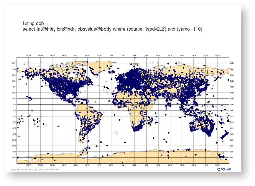
Using an ODB file and create a geographical map

In this example, we have downloaded some ODB data from Mars.

The mars request looks like:

Code Block

title	Mars request

retrieve,
    class      = e2,
    type       = ofb,
    stream     = oper,
    expver     = 1607,
    repres     = bu,
    reportype  = 16005,
    obstype    = 1,
    date       = 20100101,
    time       = 0,
    domain     = g,
    target     = "data.odb",
    filter     = "select lat@hdr, lon@hdr, obsvalue@body where (source='ispdv2.2') and (varno=110)",
    duplicates = keep

We retrieve 3 columns lat@hdr, lon@hdr, obsvalue@body. In that case obsvalue@body will contain the value of the Surface pressure in Pascal.

We can dump the result :

Code Block

title	odb ls

lat@hdr         lon@hdr         obsvalue@body
84.559998       -44.100006      100180.000000
84.349998       -46.989990      100140.000000
83.610001       -89.299988      100380.000000
83.419998       -71.970001      100140.000000
83.300003       -69.040009      100090.000000
82.480003       -93.190002      100350.000000
82.449997       -170.309998     101510.000000
82.260002       -128.949997     99180.000000
81.449997       -144.850006     100180.000000
81.419998       -144.619995     100180.000000
81.400002       -145.550003     100250.000000
80.709999       -110.500000     100180.000000
80.320000       -179.860001     102969.992188
80.019997       -151.399994     100440.000000

In this example, we will ask Magics to load this ODB file, and plot the position of each observation using the simple marker. WE have to inform Magics about the name of the columns to use to find the latitude, and longitude information.

Section

Column

width	350px

Column

width	70%

Code Block

language	py
title	Simple symbol plotting
collapse	true

# importing Magics module
from Magics.macro import *

# Setting of the output file name
output = output(output_formats=['png'],
                output_name_first_page_number='off',
                output_name="odb_step1")

# Background Coastlines
background = mcoast(
    map_coastline_sea_shade_colour='white',
    map_coastline_land_shade_colour='cream',
    map_grid='on',
    map_coastline_land_shade='on',
    map_coastline_sea_shade='on',
    map_label='on',
    map_coastline_colour='tan',
    )
# Import odb data
odb = odb_geopoints(odb_filename='geo.odb',
                    odb_latitude_variable='lat@hdr',
                    odb_longitude_variable='lon@hdr',
                    )
# Define the symbol plotting
symbol = msymb(symbol_type='marker',
               symbol_colour='navy',
               symbol_marker_index=3,
               symbol_height=0.4,
            )
# Add a title 
lines = ['Using odb...', 
         'select lat@hdr, lon@hdr, obsvalue@body where (source='ispdv2.2') and (varno=110)',
         ]

title = mtext(
    text_lines=lines,
    text_justification='left',
    text_font_size=0.7,
    text_colour='charcoal',
)

#Create the plot
plot(output, background, odb, symbol, title)

Now, we are going to colour the symbol according to the value of the observation. The advanced mode for symbol plotting offers an easy way to specify range and colours, we add a legend for readability.

Section

Column

width	350px

Column

width	70%

Code Block

language	py
title	Advanced symbol plotting
collapse	true

# importing Magics module
from Magics.macro import *

# Setting of the output file name
output = output(output_formats=['png'],
                output_name_first_page_number='off',
                output_name='odb_step2')

# Background Coastlines
background = mcoast(
    map_coastline_sea_shade_colour='white',
    map_coastline_land_shade_colour='cream',
    map_grid='on',
    map_coastline_land_shade='on',
    map_coastline_sea_shade='on',
    map_label='on',
    map_coastline_colour='tan',
    )

# Import odb data
odb = odb_geopoints(odb_filename='geo.odb',
                    odb_latitude_variable='lat@hdr',
                    odb_longitude_variable='lon@hdr',
                    odb_value_variable='obsvalue@body',
                    )

# Define the symbol plotting
symbol = msymb(symbol_type='marker',
               symbol_colour='navy',
               symbol_advanced_table_selection_type='list',
               symbol_advanced_table_level_list=[50000., 75000., 90000., 100000., 100500., 101000., 101500., 102000., 102500., 103000., 103500., 104000., 105000.],
               symbol_advanced_table_min_level_colour='blue',
               symbol_advanced_table_max_level_colour='red',
               symbol_advanced_table_colour_direction='clockwise',
               symbol_table_mode='advanced',
               legend='on'
               )
#Adding some text
lines = ['Using odb colouring the sumbol according to the value of the observation...', "select lat@hdr, lon@hdr, obsvalue@body where (source='ispdv2.2') and (varno=110)",
         '<magics_title/>']

title = mtext(
    text_lines=lines,
    text_html='true',
    text_justification='left',
    text_font_size=0.7,
    text_colour='charcoal',
    )

#adding some legend
legend = mlegend(legend='on', legend_text_colour='navy',
                 legend_display_type='continuous')


#Create the plot
plot(output, background, odb, symbol, title,legend)

Space shortcuts

Page tree

Versions Compared

Old Version 11

New Version 12

Key

Using an ODB file and create a geographical map