VAPOR
The home of the software is https://www.vapor.ucar.edu :
...
What is VAPOR?
VAPOR stands for Visualization and Analysis Platform for Ocean, Atmosphere, and Solar Researchers. It
...
is a software system providing an interactive 3D visualization environment that runs on most UNIX, Windows and Mac systems equipped with modern 3D graphics cards.
VAPOR is designed to handle WRF output files. To handle ECMWF GRIB output a conversion is required.
VAPOR data files
VAPOR input data is described by .vdf (VAPOR data Format) files. These are XML files containing the name and dimension all the variables and the path of the actual data files storing the data values. VAPOR stores its actual data values in .vdc (VAPOR Data Collection) files. These are NetCDF files containing wavelet compressed 3D data. There is a separate file for each variable and timestep organized into a folder hierarchy.
The input data must be defined on a 3D grid, which has to be regular horizontally. Vertically the grid can be:
- equidistant (regular)
- layered. For layered grids the elevation above sea level of each layer should be available as a variable called ELEVATION. VAPOR can then use it to interpolate all the data to height levels internally.
- spherical
VAPOR uses a right-handed coordinate system which means that :
- the horizontal grid has to start at the SW corner
- the vertical coordinates have to increase along the z axis (upwards).
How to generate input data at ECMWF?
There are two possible ways.
The first way is to convert GRIB to NetCDF and then convert it to VAPOR format by the ncdf2vdf VAPOR command line tool.
| Gliffy Diagram | ||
|---|---|---|
|
The other way is to dump gridded data to a raw binary format that can be convert to VAPOR format by the raw2vdf VAPOR command line tool.
| Gliffy Diagram | ||
|---|---|---|
|
An example for data generation
The easiest way is to use pressure level data from MARS. These are the steps involved:
1.Retrieve data from MARS:
- 2D (surface): z, 2t, msl, ...
- 3D (pressure levels): z, t, ...
At this point the start point of the grid is at NW!
2. Process each timestep independently (all can be done in a Macro):
- rearrange the grid so that start point should be at SW
- change z units to m
- change temperature units to C
- derive wind speed filelds
- create one GRIB file for the 2D and another one for the 3D variables
- call the grib_to_netcdf GRIB API command to generate netCDF data from both files
- call the ncrename NCO command to change the name of the surface and pressure level geopotential to HGT and ELEVATION, respectively. This latter is required by VAPOR. (To make this work we need to 'use nco' before stating up Metview.)
This is the Macro code that was written to perform all these tasks to generate dataset for the Hurricane Sandy case.
| Code Block | ||
|---|---|---|
| ||
#Metview Macro

# **************************** LICENSE START ***********************************
#
# Copyright 2013 ECMWF. This software is distributed under the terms
# of the Apache License version 2.0. In applying this license, ECMWF does not
# waive the privileges and immunities granted to it by virtue of its status as
# an Intergovernmental Organization or submit itself to any jurisdiction.
#
# ***************************** LICENSE END ************************************

g2Inp=read("sandy_surf.grib")
g3Inp=read("sandy_upper_pl.grib")


#Specify outdir
outDir = "sandy_data_pl"
if not(exist(outDir)) then
  	shell("mkdir -p " & outDir)
end if


#Define variable list
v2Lst=["2t","10u","10v","msl","z","sstk"]
v3Lst=["z","t","r","u","v","w","pv"]

#Define steps
stepLst=nil
for i=0 to 120 by 12 do
	stepLst=stepLst & [i]
end for


#Processing steps
for i=1 to count(stepLst) do


	step=stepLst[i]


	#---------------------------------------

	# 2D -- change geopotential to height

	#---------------------------------------


	gRes=nil

	loop v in v2Lst

			g=read(step: step, param: v, data: g2Inp)

			if v = "z" then

				g=g/9.81

				#g=grib_set_string(g,["shortName","HGT"])

			end if

			if v = "2t" or v ="sstk" then

				g=g-273.1

			end if

			gRes = gRes & reorientGrid(g)

	end loop


	u=read(step: step, param: "10u", data: gRes)

	v=read(step: step, param: "10v", data: gRes)

	sp=sqrt(u*u+v*v)

	sp=grib_set_string(sp,["shortName","10si"])

	gRes = gRes & sp


	#Convert 2d data to netcdf

	grbName=outDir & "/surf_tmp.grb"

	write(grbName,gRes)

	ncName=outDir & "/sandy_2D." & step & ".nc"

	shell("grib_to_netcdf -D NC_FLOAT -o " & ncName & " " & grbName)

	shell("ncrename -vz,HGT " & ncName)


	#---------------------------------------

	# 3D -- interpolate to height levels

	#---------------------------------------


	gRes=nil


	#Get geopotemtial

	#z=read(step: step, param: "z", data: g3Inp)


	loop v in v3Lst

			g=read(step: step, param: v, data: g3Inp)

			if v = "z" then

				g=g/9.81

				#g=grib_set_string(g,["shortName","ELEVATION"])

			end if

			if v = "t" then

				g=g-273.1

			end if

			gRes = gRes & reorientGrid(g)

	end loop


	u=read(step: step, param: "u", data: gRes)

	v=read(step: step, param: "v", data: gRes)

	sp=sqrt(u*u+v*v)

	sp=grib_set_string(sp,["shortName","ws"])

	gRes = gRes & sp


	#Convert 3d data to netcdf

	grbName=outDir & "/upper_tmp.grb"

	write(grbName,gRes)

	ncName=outDir & "/sandy_3D." & step & ".nc"

	shell("grib_to_netcdf -D NC_FLOAT -o " & ncName & " " & grbName)

    shell("ncrename -vz,ELEVATION " & ncName)


end for


function reorientGrid(f)


	res=nil


	loop g in f


	latScan=grib_get_long(g,"jScansPositively")

	if latScan = 0 then

		lat1=grib_get_double(g,"latitudeOfFirstGridPointInDegrees")

		lat2=grib_get_double(g,"latitudeOfLastGridPointInDegrees")


		lon1=grib_get_double(g,"longitudeOfFirstGridPointInDegrees")

		lon2=grib_get_double(g,"longitudeOfLastGridPointInDegrees")


		v=values(g)

		nx=grib_get_long(g,"Ni")

		ny=grib_get_long(g,"Nj")


		vn=vector(nx*ny)


		for j=1 to ny do

			for i=1 to nx do

			  vn[(j-1)*nx+i]=v[(ny-j)*nx+i]

			end for

		end for


		g=grib_set_double(g,["latitudeOfFirstGridPointInDegrees",lat2,

		                     "latitudeOfLastGridPointInDegrees",lat1])


		g=grib_set_double(g,["longitudeOfFirstGridPointInDegrees",lon1-360,

		                     "longitudeOfLastGridPointInDegrees",lon2-360])


		g=grib_set_long(g,["jScansPositively",1])

		g=set_values(g,vn)


	end if


	res = res &	g


   end loop


   return res


end reorientGrid |
3. Create a vdf file width VAPOR command vdfcreate (in a shell script):
| Code Block |
|---|
#Writing user times into a file
startTime=988968
tstr=$startTime
for ((t=1; t<$num_timesteps; t++))
do
    tstr=${tstr}" "$((startTime + t*12))
done
echo $tstr  > tsfile.txt

#Defining lat lon corners in vapor units = metres from point (0,0)
latS=$((15*111177))
latN=$((57*111177))
lonW=$((-101*111177))
lonE=$((-39*111177))

#Create the vdf file
vdfcreate -dimension 249x169x20 \
          -gridtype layered \
          -mapprojection "+proj=latlong  +ellps=sphere" \
          -level 2 \
          -usertimes tsfile.txt \
          -extents ${lonW}:${latS}:0:${lonE}:${latN}:16000  \
          -vars3d t:r:pv:u:v:w:ws:ELEVATION \
          -vars2dxy HGT:v2t:sst:msl:v10u:v10v:v10si \
          $file_prefix.vdf

for ((t=0; t<$num_timesteps; t++))
do
    tLabel=$((t*12))
    echo $tLabel

    #-startts $t

    ncdf2vdf -vars HGT:v2t:sst:msl:v10u:v10v:v10si -timedims time -timevars time -numts 1 sandy_2D.${tLabel}.nc  $file_prefix.vdf
    ncdf2vdf -vars t:r:pv:u:v:w:ws:ELEVATION -timedims time -timevars time -numts 1 sandy_3D.${tLabel}.nc  $file_prefix.vdf

done |
Here we have to define the grid dimensions, the number of timesteps, the coordinate range and the 2 and 3d variables. If we want to enable georeferencing for our data in VAPOR we need to set the map projection correctly as well using the PROJ4 syntax and units. We also needed to create an ASCII file containing the all the time values (this step is needed because we have all timesteps in separate files).
4. Load the netcdf data into VAPOR with command ncdf2vdf (in a shell script):
| Code Block |
|---|
for ((t=0; t<$num_timesteps; t++))
do
    tLabel=$((t*6))

    ncdf2vdf -vars h:v2t:sst:msl:v10u:v10v -timedims time -timevars time -numts 1 sandy_2D.${tLabel}.nc  res.vdf
    ncdf2vdf -vars t:r:pv:u:v:w -timedims time -timevars time -numts 1 sandy_3D.${tLabel}.nc  res.vdf

done |
IFS example dataset
The VAPOR dataset derived with the macro and script above can be find at:
/scratch/graphics/cgr/vapor/sandy_pl
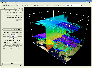
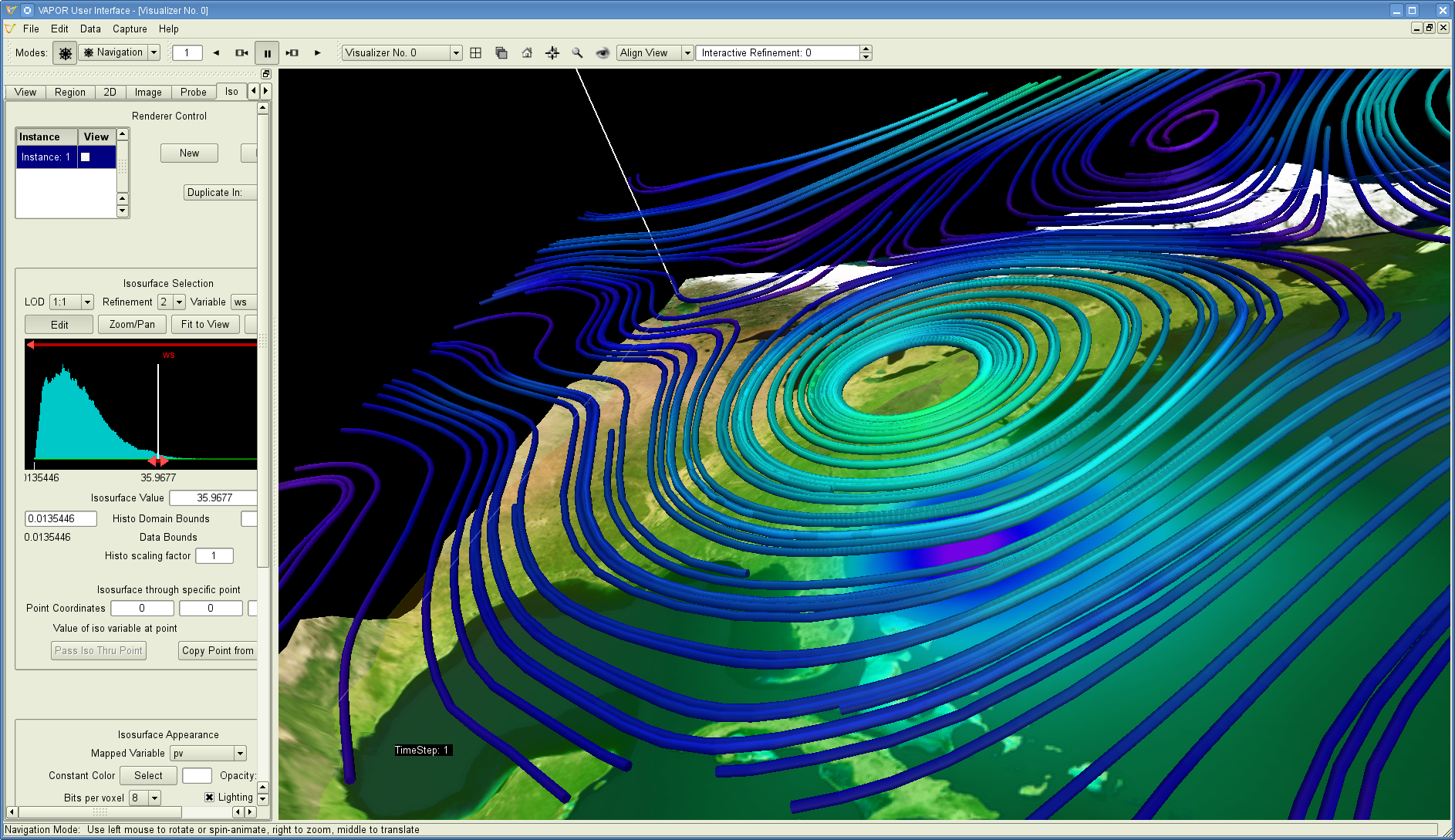
Here are some snapshots created with this data:


Starting up VAPOR
To set up for running, source either
/scratch/graphics/cgm/vapor/vapor-2.2.2/bin/vapor-setup.csh
or
/scratch/graphics/cgm/vapor/vapor-2.2.2/bin/vapor-setup.csh
This sets up the path, etc so we can then run
vaporgui
Using VAPOR
session files (.vss)
transfer function files (.vtf)
Python interface:
http://www.vapor.ucar.edu/page/using-python-vapor
Geotiff
see how to geotiff images generated by NCL inVAPOR:
http://www.ncl.ucar.edu/Applications/wrfvapor.shtml
or
http://www.vapor.ucar.edu/page/ncl-and-vapor
Problems/questions
- How to display time stamp?
How to prepare ECMWF model output for visualisation in VAPOR?
(following instructions were provided by Marc Rautenhaus, TU München, Germany, May 2013)
I have put together a couple of my scripts and some grib files to
(hopefully) working example of how I convert ECMWF forecasts to the
Vapor data format. Feel free to forward this email to anyone of your
group, I'd just like to ask you to not distribute the code in the example.
You can download the archive here:
https://gigamove.rz.rwth-aachen.de/d/id/meqWwxJwmGx7n7
The archive contains a /data directoy containing a few grib files of the
deterministic forecast during T-NAWDEX (October 2012). The file contain
forecast timesteps 0-36h and the lowest 72 model levels (up to ~10hPa).
In the /script directory are some example scripts that convert the data
to Vapor VDF. Please have a look at the README file, in which I have
described what the scripts are doing and how to use them. To run the
example, you need to have Vapor 2.1 installed (I assume it will also run
with 2.2, but I haven't tested that yet). It also requires
netcdf4python. Three scripts convert the grib files to NetCDF, compute
some additional variables and convert the NetCDF data into VDF. You need
to change some paths hard-coded into the scripts, see the README file.
Note that the scripts are "hand-made" for the specific dataset. The
/mslib subdirectory contains parts of the MSS. The "ppecmwf" tool is a
Python tool that I have written to perform computations on ECMWF data in
NetCDF format.
Additonally, I've put the code that I use operationally on the MSS
server into the /metdp directory. This code won't run out of the box,
but you can have a look at it to see how the conversion to VDF is done
there. It is basically the same as in the example scripts but
implemented in Python and not restricted to a specific dataset. The
important class is met_data_processor.py/ECMWF_NetCDF_to_VDF_DIP.
I hope the example will be useful for you. If you have any questions
just let me know.
Marc
You can read the README file with instruction by
nedit /scratch/graphics/cgm/vapor/ecmwf_vapor_tutorial/1_simple_36h/scripts/README
The home of the software is https://www.vapor.ucar.edu.
How to use VAPOR with Metview?
VAPOR has its own internal data model and NWP data has to be converted into the VAPOR format. There are a set of VAPOR command line tools that can convert NetCDF input data into this format but there is no such tool available for GRIB.
Metview's VAPOR Prepare icon helps to overcome this difficulty and allows converting GRIB data into the VAPOR format.

Once the conversion has been completed the VAPOR Prepare icon can be used to start up VAPOR to provide interactive 3D visualisation for the data. The snapshots below show how ECMWF data is actually displayed in VAPOR.
Further details
There is a tutorial available on the use of VAPOR with Metview. It explains both the data preparation steps and the basics of the visualisation.
| Excerpt | ||
|---|---|---|
|
...