Download the initial data
| HTML |
|---|
<ol> <li>Navigate to the <a href="http://download.ecmwf.int/test-data/openifs/reference_casestudies" target="_blank">http://download.ecmwf.int/test-data/openifs/reference_casestudies</a> site in a web browser, choose the experiment initialized from ERA5 data on 3 December 2015 with T255L91 resolution (i.e., <span class="font_code_black">gs0c</span> experiment) and download the .gz file (approximately 128 MB) into the <span class="font_code_black">data/initial_conditions/gs0c</span> directory. Or from the command line: |
| Code Block |
|---|
% cd data/initial_conditions/gs0c % wget -c http://download.ecmwf.int/test-data/openifs/reference_casestudies/data/Desmond_201512/T255L91_ERA5/gs0c_2015120300.tar.gz |
| HTML |
|---|
</li><li number=2>To unpack the files either use the <span class="font_code_black">tar -zxf</span> command if your version of <span class="font_code_black">tar</span> supports the '<span class="font_code_black">z</span>' option: |
| Code Block |
|---|
% tar -zxf gs0c_2015120300.tar.gz |
or use gunzip followed by tar -xf:
| Code Block |
|---|
% gunzip gs0c_2015120300.tar.gz % tar -xf gs0c_2015120300.tar |
| HTML |
|---|
</li></ol> |
Prepare the experiment
Go to the working directory where your experiment will run and clean it if it has been already used:
Code Block % cd ${OIFS_HOME}/rundir % rm -f ICM* ifsdata rtables *l_2 wam* *in fort.* master.exe MPP*Copy or link the initial conditions from the input directory to your working directory:
Code Block % INPUTDIR=${OIFS_HOME}/data/initial_conditions/gs0c % ln -sf ${INPUTDIR}/ICM* . % ln -sf ${INPUTDIR}/wam* . % ln -sf ${INPUTDIR}/*in .- Set the necessary environment variables:
- OIFS_GRIB_API_DIR: folder of GRIB-API
- OIFS_DATA_DIR: folder of climate data called ifsdata
- LD_LIBRARY_PATH: folder of GRIB_API libraries
- GRIB_SAMPLES_PATH: path of GRIB_API samples
Copy the namelists to your rundir:
Code Block % NAMDIR=${OIFS_HOME}/data/initial_conditions/gs0c % cp ${NAMDIR}/wam_namelist . % cp ${NAMDIR}/wam_namelist_coupled_000 . % cp ${NAMDIR}/namelistfc fort.4Modify the fort.4 file with setting the following namelist variables:
Number of processors you use to run OpenIFS: NPROC in the NAMPAR0 group,
- Set the NPRNT_STATS (in the NAMPAR0 group) to the same value as NPROC,
- Timestep: TSTEP=2700 in the NAMDYN group,
- Number of vertical levels and spectral truncation: NFPLEV=91 and NFPMAX=255 in the NAMFPG group,
- Experiment ID: CNMEXP="gs0c" in the NAMCT0 group,
Number of latitudes and longitudes on the transform grid: NLAT=256, NLON=512 in the NAMFPD group,
HTML Fullpos variables in the <span class="font_code_black">NAMFPC</span> group (for more details please see <a href="https://software.ecmwf.int/wiki/display/OIFS/6.2+Model+experiments#id-6.2Modelexperiments-Thenamelist" target="_blank">section 6.2</a>),
Output file names: setting LINC="true" in the NAMOPH group leads to ICM??${expID}+00${step} output file names where step is in hour instead of timestep (here on 4 digits).
Run the model using the oifs_run.sh script which is in the OpenIFS 40r1v2 package. To run the script you have to specify the experiment ID, the executable file (named master.exe), the forecast length and you can set the spectral truncation as well as the timestep here:
Code Block % # oifs_run.sh -e${expID} -m${executable} -r${RESOUTION} -f${SCLENGTH} -s${TSTEP} % ${JOBDIR}/oifs_run.sh -egs0c -m${BINDIR}/master.exe -r255 -fh96 -s2700 > out 2>errWith these settings you run a 96-hour forecast (-fh96), where JOBDIR and BINDIR are the location of the oifs_run.sh script and the master.exe OpenIFS executable, respectively.
Before the model run begins, the oifs_run.sh script checks the inputs and ensure that the necessary climate data on the corresponding resolution are also available in your working directory.When OpenIFS starts to run, you will see the following content in your working directory:
Code Block master.exe fort.4 # executable and namelist wam_namelist wam_namelist_coupled_000 # namelists for the wave model ICMGGgs0cINIUA ICMCLgs0cINIT ICMSHgs0cINIT ICMGGgs0cINIT # initial conditions cdwavein sfcwindin specwavein uwavein # wave model initial conditions wam_grid_tables wam_subgrid_0 wam_subgrid_1 wam_subgrid_2 # wave model files ifsdata rtables 255l_2 # climate data ncf927 ifs.stat NODE.001_01 # text output (log) files out err # output and error files from the model run ICMGGgs0c+000000 ICMSHgs0c+000000 ICMGGgs0c+000003 ICMSHgs0c+000003 # output files for the first two steps
HTML For more information about the content of the working directory, please see <a href="https://software.ecmwf.int/wiki/display/OIFS/6.2+Model+experiments#id-6.2Modelexperiments-Downloadingtheinputdata" target="_blank">section 6.2</a>.
| HTML |
|---|
<p>For more instructions and details about running the model, please visit the related <a href="https://software.ecmwf.int/wiki/display/OIFS/5.6+Acceptance+testing+OpenIFS+after+installation" target="_blank">page</a> in the <a href="https://software.ecmwf.int/wiki/display/OIFS/OpenIFS+User+Guides" target="_blank">OpenIFS User Guides</a>.</p> |
Post-processing the model outputs
The Metview macros prepared for visualization of experiment results require the meteorological variables in GRIB format separated by variables and days with the appropriate names.
The 2-meter temperature, the precipitation, the mean sea level pressure and the wind gust are expected in gridpoint representation. They are prepared from the ICMGG* outputs with the next operations:
Code Block % expID=gs0c; date=20151203 % steps="00 03 06 09 12 15 18 21 24 27 30 33 36 39 42 45 48 51 54 57 60 63 66 69 72" # every 3 hours from 0 UTC on 3 December to 0 UTC on 6 December % for step in ${steps} do grib_copy -w shortName=2t ICMGG${expID}+0000${step} t2_${date}_${step}.grib #to get the 2-meter temperature grib_copy -w shortName=msl ICMGG${expID}+0000${step} mslp_${date}_${step}.grib #to get the mean sea level pressure grib_copy -w shortName=10fg ICMGG${expID}+0000${step} gust_${date}_${step}.grib #to get the 10-meter wind gust doneFor precipitation, both the convective and large-scale precipitation components have to be gathered in the same file:
Code Block % expID=gs0c; date=20151203 % steps="00 03 06 09 12 15 18 21 24 27 30 33 36 39 42 45 48 51 54 57 60 63 66 69 72" # every 3 hours from 0 UTC on 3 December to 0 UTC on 6 December % for step in ${steps} do grib_copy -w shortName=lsp/cp ICMGG${expID}+0000${step} p_${date}_${step}.grib doneThe pressure level data are required in spectral representation. They are prepared from the ICMSH* outputs with the next operations:
Code Block % expID=gs0c; date=20151203 % steps="00 03 06 09 12 15 18 21 24 27 30 33 36 39 42 45 48 51 54 57 60 63 66 69 72" # every 3 hours from 0 UTC on 3 December to 0 UTC on 6 December % for step in ${steps} do grib_copy -w shortName=t,level=850 ICMSH${expID}+0000${step} t850_${date}_${step}.grib #to get the temperature at 850 hPa grib_copy -w shortName=r,level=700 ICMSH${expID}+0000${step} q700_${date}_${step}.grib #to get the relative humidity at 700 hPa grib_copy -w shortName=z,level=500 ICMSH${expID}+0000${step} z500_${date}_${step}.grib #to get the geopotential at 500 hPa doneFor wind, both the u and v components have to be collected in the same file:
Code Block % expID=gs0c; date=20151203 % steps="00 03 06 09 12 15 18 21 24 27 30 33 36 39 42 45 48 51 54 57 60 63 66 69 72" # every 3 hours from 0 UTC on 3 December to 0 UTC on 6 December % for step in ${steps} do grib_copy -w shortName=u/v,level=250 ICMSH${expID}+0000${step} u250_${date}_${step}.grib #to get the u and v components at 250 hPa grib_copy -w shortName=u/v,level=100 ICMSH${expID}+0000${step} u100_${date}_${step}.grib #to get the u and v components at 100 hPa doneAfter these operations, the timesteps belonging to the same days have to be merged into a common file and the concatenated file has to be moved to the input directory of the Metview visualization:
Code Block % expID=gs0c; date=20151203 % variables="t2 mslp gust p t850 q700 z500 u250 u100" % for variable in ${variables} do cat ${variable}_${date}_*.grib > ${variable}_${date}.grib mv ${variable}_${date}.grib ${OIFS_HOME}/data/${expID} done
| HTML |
|---|
<p>More details can be found about the post-processing in <a href="https://software.ecmwf.int/wiki/display/OIFS/6.3+Data+pre-processing+for+visualization#id-6.3Datapre-processingforvisualization-Post-processingofmodeloutputs" target="_blank">section 6.3</a>.</p> |
Download the re-analysis data
As reference for the evaluation, we use both ERA-Interim and ERA5 re-analyses. The data are provided on the ECMWF download server in the proper format needed for visualization with Metview or they can be downloaded in their original format from the ECMWF MARS system. This retrieve has to be accomplished only once, if we download the data for the whole period of the case study.
To download the re-analysis GRIB files from the download server into the input directory of the Metview visualization:
| Code Block | ||
|---|---|---|
| ||
% cd ${OIFS_HOME}/data/reference
% wget -c http://download.ecmwf.int/test-data/openifs/reference_casestudies/data/Desmond_201512/reference/ei_20151201-20151206.tar.gz # ERA-Interim
% wget -c http://download.ecmwf.int/test-data/openifs/reference_casestudies/data/Desmond_201512/reference/ea_20151201-20151206.tar.gz # ERA5 |
| Expand | ||||||||||||||||||||||||||||||||||||
|---|---|---|---|---|---|---|---|---|---|---|---|---|---|---|---|---|---|---|---|---|---|---|---|---|---|---|---|---|---|---|---|---|---|---|---|---|
| ||||||||||||||||||||||||||||||||||||
|
| HTML |
|---|
<p>More information is provided about the background of the different re-analyses in <a href="https://software.ecmwf.int/wiki/display/OIFS/6.3+Data+pre-processing+for+visualization#id-6.3Datapre-processingforvisualization-Preparationofreferencedata" target="_blank">section 6.3</a>.</p> |
Plotting
| HTML |
|---|
<p>The visualization package is available in the <span class="font_code_black">casestudies</span></a> directory of the OpenIFS cycle 40r1v2 release as well as in the ECMWF download server: <a href="http://download.ecmwf.int/test-data/openifs/reference_casestudies/programs/metview/" target="_blank">http://download.ecmwf.int/test-data/openifs/reference_casestudies/programs/metview</a>. Transfer the content of the <span class="font_code_black">definitions</span> and <span class="font_code_black">macros</span> folders into the corresponding local directories. Going to the <span class="font_code_black">macros</span> folder, the visualization can be done by the Metview macros (<span class="font_code_black">*.mv</span> files) in two ways: (1) interactively using a dialogue box or (2) in batch mode.</p> <p>Before using the macros, the path of the <span class="font_code_black">definitions</span> directory has to be added to the <span class="font_code_black">METVIEW_MACRO_PATH</span> to reach the external functions and colour definitions:</p> |
| Code Block |
|---|
% cd ${OIFS_HOME}/macros
% export METVIEW_MACRO_PATH="${OIFS_HOME}/definitions:${METVIEW_MACRO_PATH}" |
There is an include statement in the plot_forecastrun.mv and plot_ERAI_ERA5.mv macros and further 2 ones in plot_IC.mv taking the two colour definitions from this directory. The path of the definitions folder has to be set in the macros according to the local working tree. To do that, open these files in a text editor, search the definitions and modify its path if it is necessary (4 times in total).
(1) Interactive plotting
Forecast maps
| Expand | ||
|---|---|---|
| ||
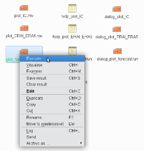
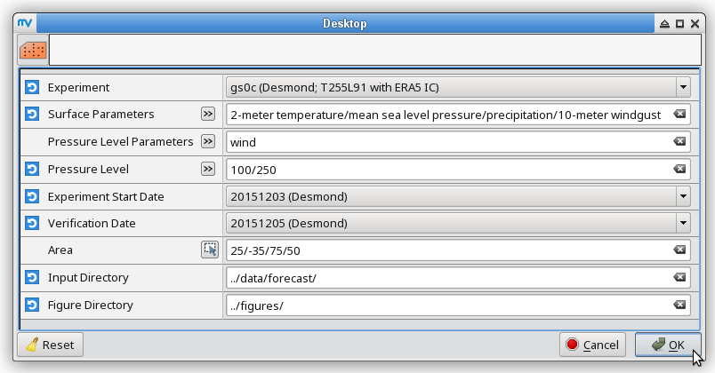
To prepare maps from the T255L91 forecast initialized with ERA5 on 3 December 2015 for the validation date, i.e., 5 December 2015, start Metview (just type metview and press Enter), execute plot_forecastrun.mv with right mouse click on its icon and selecting the
These steps generate all the maps from the forecast outputs between 0 UTC on 5 December and 0 UTC on 6 December. |

Re-analysis maps
| Expand | ||
|---|---|---|
| ||
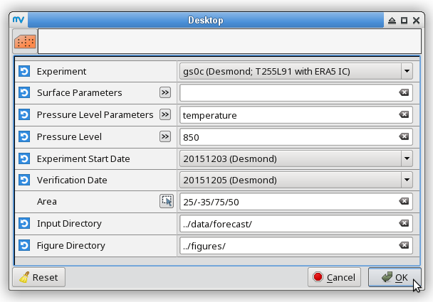
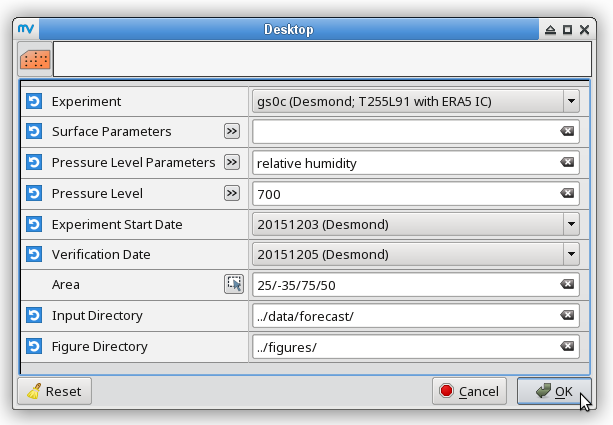
The time handling in case of the re-analyses is different, so the procedure to prepare maps from the ERA-Interim data for the validation date consists of the following steps:
To prepare maps from the ERA5 data for the validation date, repeat the steps 1 to 3 above selecting ERA5 as reference (below an example for the temperature at 850 hPa):
|

Maps from the initial conditions
| Expand | |||||
|---|---|---|---|---|---|
| |||||
To compare the initial conditions with the ones of the T255L91 experiment initialized from ERA-Interim (with gryg experiment ID) on 3 December 2015, you do not have to run the latter experiment because only the initial conditions are needed.
|
(2) Plotting in batch mode
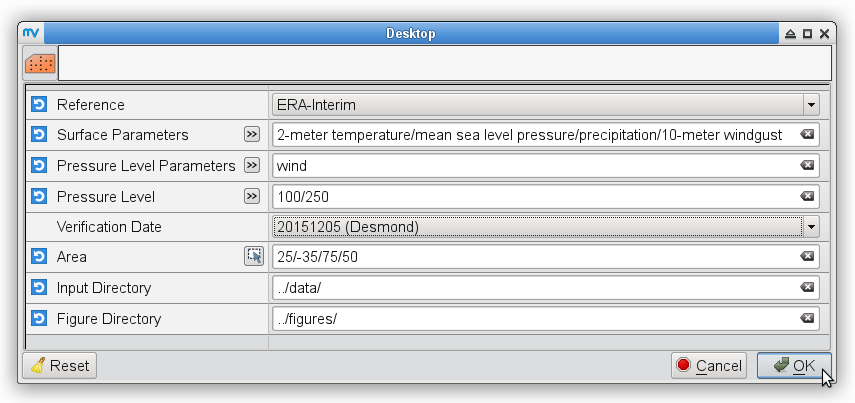
To prepare maps from the T255L91 forecast initialized with ERA5 on 3 December 2015 for the validation date, i.e., 5 December 2015:
Code Block % # metview -b plot_forecastrun.mv [experiment_ID] [resolution] [initial_condition] \ % # [parameters] [pressure_levels] [start_date] [verification_date] \ % # [area] [input_directory] [output_directory] % metview -b plot_forecastrun.mv gs0c T255L91 ea "t2,mslp,p,gust" " " 20151203 20151205 "25,-35,75,50" ../data/forecast/ ../figures/ # surface parameters % metview -b plot_forecastrun.mv gs0c T255L91 ea "t" "850" 20151203 20151205 "25,-35,75,50" ../data/forecast/ ../figures/ # t850 % metview -b plot_forecastrun.mv gs0c T255L91 ea "q" "700" 20151203 20151205 "25,-35,75,50" ../data/forecast/ ../figures/ # q700 % metview -b plot_forecastrun.mv gs0c T255L91 ea "z" "500" 20151203 20151205 "25,-35,75,50" ../data/forecast/ ../figures/ # z500 % metview -b plot_forecastrun.mv gs0c T255L91 ea "u" "250,100" 20151203 20151205 "25,-35,75,50" ../data/forecast/ ../figures/ # u250, u100
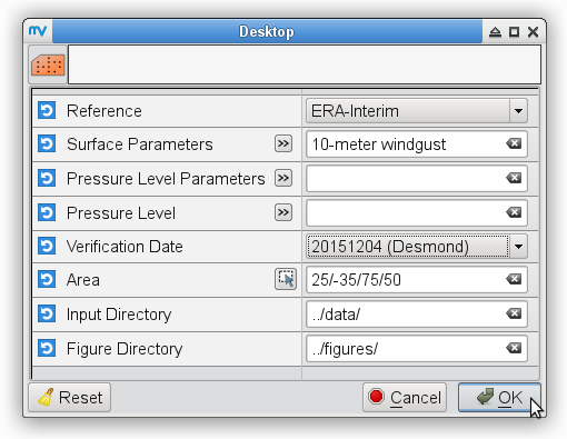
To prepare maps from the ERA-Interim data for the validation date:
Code Block % # metview -b plot_forecastrun.mv [reference] [parameters] [pressure_levels]\ % # [verification_date] [area] [input_directory] [output_directory] % for date in 20151205 20151206 do metview -b plot_ERAI_ERA5.mv ERA-Interim "t2,mslp" " " ${date} " " ../data/ ../figures/ # surface parameters metview -b plot_ERAI_ERA5.mv ERA-Interim t 850 ${date} " " ../data/ ../figures/ # t850 metview -b plot_ERAI_ERA5.mv ERA-Interim q 700 ${date} " " ../data/ ../figures/ # q700 metview -b plot_ERAI_ERA5.mv ERA-Interim z 500 ${date} " " ../data/ ../figures/ # z500 metview -b plot_ERAI_ERA5.mv ERA-Interim u "250,100" ${date} " " ../data/ ../figures/ # u250, u100 done % metview -b plot_ERAI_ERA5.mv ERA-Interim "p" " " 20151205 " " ../data/ ../figures/ # precipitation % metview -b plot_ERAI_ERA5.mv ERA-Interim "gust" " " 20151204 " " ../data/ ../figures/ # windgustTo prepare maps for the validation date, i.e., 5 December 2015 from the ERA5 data:
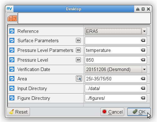
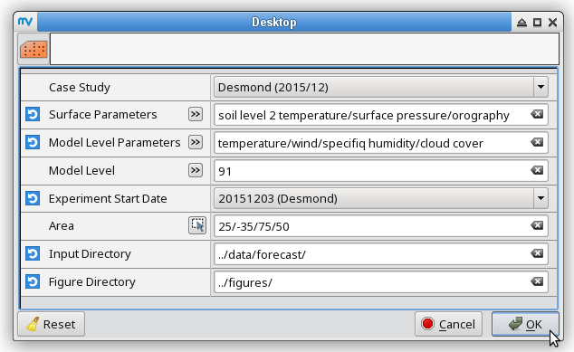
Code Block % for date in 20151205 20151206 do metview -b plot_ERAI_ERA5.mv ERA5 "t2,mslp" " " ${date} " " ../data/ ../figures/ # surface parameters metview -b plot_ERAI_ERA5.mv ERA5 t 850 ${date} " " ../data/ ../figures/ # t850 metview -b plot_ERAI_ERA5.mv ERA5 q 700 ${date} " " ../data/ ../figures/ # q700 metview -b plot_ERAI_ERA5.mv ERA5 z 500 ${date} " " ../data/ ../figures/ # z500 metview -b plot_ERAI_ERA5.mv ERA5 u "250,100" ${date} " " ../data/ ../figures/ # u250, u100 done % metview -b plot_ERAI_ERA5.mv ERA5 "p" " " 20151205 " " ../data/ ../figures/ # precipitation % metview -b plot_ERAI_ERA5.mv ERA5 "gust" " " 20151204 " " ../data/ ../figures/ # windgustTo compare the initial conditions with the ones of the T255L91 experiment initialized from ERA-Interim (with gryg experiment ID) on 3 December 2015, you do not have to run the latter experiment because only the initial conditions are needed. Before running the macro plot_IC.mv, we have to copy the initial conditions into the corresponding input directory and append a suffix with the appropriate date to the filename:
Code Block % expIDs="gryg gs0c" % for expID in $expIDs; do for file in ICMGG${expID}INIT ICMSH${expID}INIT ICMGG${expID}INIUA; do cp ${OIFS_HOME}/data/initial_conditions/${expID}/2015120300/${file} ${OIFS_HOME}/data/forecast/${expID}/${file}_20151203 done done % # metview -b plot_IC.mv [case_study] [parameters] [model_levels]\ % # [start_date] [area] [input_directory] [output_directory] % metview -b plot_IC.mv Desmond "t2,mslp,p,gust" " " 20151203 "25,-35,75,50" ../data/forecast/ ../figures/ # surface parameters % metview -b plot_IC.mv Desmond t 850 20151203 "25,-35,75,50" ../data/forecast/ ../figures/ # t850 % metview -b plot_IC.mv Desmond q 700 20151203 "25,-35,75,50" ../data/forecast/ ../figures/ # q700 % metview -b plot_IC.mv Desmond z 500 20151203 "25,-35,75,50" ../data/forecast/ ../figures/ # z500 % metview -b plot_IC.mv Desmond u "250,100" 20151203 "25,-35,75,50" ../data/forecast/ ../figures/ # u250, u10
| HTML |
|---|
<p>More details about plotting with Metview are available in <a href="https://software.ecmwf.int/wiki/display/OIFS/6.4+Visualization+with+Metview" target="_blank">section 6.4</a>.</p> |
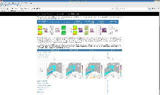
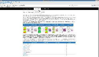
Construct the catalogue
Running the Metview macros results in a large amount of figures. The individual pictures can be assembled into a catalogue containing all relevant plots. We provide 2 possibilities for the users, the Macro functionality of Microsoft Office Word and HTML templates, from which the latter one is introduced here:
| |||||||||||
| |||||||||||
|
| ||||||||||
|
| ||||||||||
|
| ||||||||||
|
| ||||||||||
|
| ||||||||||
|
| ||||||||||


Troubleshooting
Here some cases are collected, when the model run and the forecast evaluation can terminate with error.
Model run
| HTML |
|---|
<ul> <li class="li_withspace">The initial conditions are prepared for fix dates and spatial resolutions. Make sure that your settings coincide with that.</li> <li class="li_withspace">The initial conditions are prepared with fix experiment ID that you can identify from the file names (e.g., in <span class="font_code_black">ICMGGgs0cINIT</span> experiment ID is <span class="font_code_black">gs0c</span>). Please make sure that you use the proper <span class="font_code_black">expID</span> in the job and the namelist, too.</li> <li>Further possible issues regarding running the OpenIFS and their solution are listed in the <a href="https://software.ecmwf.int/wiki/display/OIFS/FAQ%3A+Frequently+Asked+Questions" target="_blank">OpenIFS FAQ</a>.</li> </ul> |
Visualization with Metview
| HTML |
|---|
<ul> <li class="li_withspace">If you do not find the evaluation package (basically the Metview macros) in your local computing environment, you are likely to use earlier OpenIFS version than <strong>OpenIFS40r1v2</strong>. In that case, please download and install this version from the FTP server or download the Metview macros and the corresponding macro definitions from the <a href="http://download.ecmwf.int/test-data/openifs/reference_casestudies/programs/metview" target="_blank">ECMWF download server</a>.</li> <li>Metview macros can stop with error message if not the recommended software versions are used. The supported (minimum) versions are <strong>GRIB-API 1.18.0, ecCodes 2.5.0</strong> and <strong>Metview 4.7.1</strong>.<br> Using Metview 4.7.1 or 4.7.2, the next warnings are produced: |
| Code Block | ||
|---|---|---|
| ||
macro - WARN - 20180611.125356 - Ambiguous verb: 'READ' could be: macro - WARN - 20180611.125356 - READ (METVIEW) macro - WARN - 20180611.125356 - READ (TIGGEMETVIEW) macro - INFO - 20180611.125356 - Choosing READ (METVIEW) macro - WARN - 20180611.125356 - Ambiguous verb: 'READ' could be: macro - WARN - 20180611.125356 - READ (METVIEW) macro - WARN - 20180611.125356 - READ (TIGGEMETVIEW) macro - INFO - 20180611.125356 - Choosing READ (METVIEW) macro - INFO - 20180611.125358 - Warn: Magics-warning: [NONE] is not a valid value for SUBPAGE_MAP_PROJECTION: reset to default -> [cylindrical] macro - INFO - 20180611.125358 - Warn: Magics-warning: tolerance condition error for 3.14159 -1.5708 |
| HTML |
|---|
Metview 4.8.0–4.8.5 give the following warnings: |
| Code Block | ||
|---|---|---|
| ||
macro - INFO - 20180611.125358 - Warn: Magics-warning: [NONE] is not a valid value for SUBPAGE_MAP_PROJECTION: reset to default -> [cylindrical] macro - INFO - 20180611.125358 - Warn: Magics-warning: tolerance condition error for 3.14159 -1.5708 |
| HTML |
|---|
Metview 4.8.6–5.0.3 return with the following message: |
| Code Block | ||
|---|---|---|
| ||
macro - INFO - 20180611.125358 - Warn: Magics-warning: [NONE] is not a valid value for SUBPAGE_MAP_PROJECTION: reset to default -> [cylindrical] |
| HTML |
|---|
You can neglect all these warnings, they do not influence the output figures. </li> </ul> |
Metview macros might terminate with the next message if METVIEW_MACRO_PATH is not set:
Code Block language bash macro - ERROR - 20180611.143638 - Line 2729 in 'plot_IC.mv': Function not found: build_layout_2plus1(list) metview: EXIT on ERROR (line 1), exit status 1, starting 'cleanup'
Metview macros stops with error if the include statements in the .mv files are not set properly:
Code Block language bash base_visdef: No such file or directory macro - ERROR - 20180611.144342 - Line 151: Cannot include file metview: EXIT on ERROR (line 1), exit status 1, starting 'cleanup'
HTML Metview macros partly require mandatory directory structure. The folder of the input data can be arbitrary, however, under this directory macros expect the re-analysis fields to be placed in the subdirectory named <span class="font_code_black">reference</span>, while the forecast data in the subdirectory identified with the 4-digit experiment ID (i.e., <span class="font_code_black">data/reference</span> and <span class="font_code_black">data/gs0c</span> etc.). Please make sure that the input data are stored in these folders with the proper file names (more information about the requested file names can be found in <a href="https://software.ecmwf.int/wiki/display/OIFS/6.4+Visualization+with+Metview#id-6.4VisualizationwithMetview-Inputdata" target="_blank">section 6.4</a>).
- Metview macros can fail if they refer to non-existing directories. Please make sure that folders of the input data, output figures and the macro definitions are created.
- Saving the outputs can cause surprise if you do not append "/" at the end of the path when specifying the output directory. Please use "/" at the end of the input data path, too.
Metview macros are constructed to process the data for given dates and parameters. If you use them for different dates and meteorological variables (it is easy to do that in batch mode), they will return with error message. To avoid that you can run the macros first in help mode, typing:
Code Block language bash % metview -b macroname
Please be aware that Metview macros require the input parameters in pre-defined order and number. If you do not want to specify a given parameter, use " " instead, e.g.:
Code Block language bash % metview -b plot_IC.mv Desmond "t2,mslp,p,gust" " " 20151203 "25,-35,75,50" ../data/forecast/ ../figures/
where macro plot_ic.mv is executed for surface parameters, therefore, vertical levels are not specified.
- Macro plot_IC.mv plots the initial conditions solely for the T255L91 experiments. It aborts if you try to use it for experiments with different resolution.
Preparing the catalogue
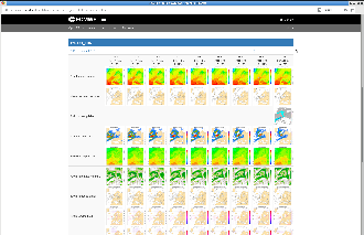
- If you want to use the prepared HTML templates to have an overview on the results, you need the pictures in .png format. Please make sure that you achieved the conversion from the .ps files.
- If none of the HTML templates show any results it is likely that you did not download and unpack them in the proper directory. Please note that it has to be done in the same folder where the .png files are located.
- If you did not conduct every experiment, HTML templates can show incomplete columns in the tables. To browse among the pictures there is no need to have all the possible figures, you can still navigate between the maps using the arrows in the top menu (after opening a picture).
| CSS Stylesheet |
|---|
.cell_nopadding {
    padding: 3px;
    border: 0px;
}

.cell_leftmargin {
    padding-left: 30px;
}

.cell_top-bottom-border {
    border-top: 1px solid #3572b0;
    border-bottom: 1px solid #3572b0;
    border-left: 0px;
    border-right: 0px;
    padding: 3px;
}

.table_noborder {
     border: 0px;
}

.vertical {
    height: 100%;
}

.vertical td:first-child {
    position: relative;
    width: 35px;
    padding: 0;
    border: 2px solid #ddd;
}

.vertical_text {
    display: block;
    white-space: nowrap;
    -moz-transform: rotate(-90deg);
    -moz-transform-origin: center center;
    -webkit-transform: rotate(-90deg);
    -webkit-transform-origin: center center;
    -ms-transform: rotate(-90deg);
    -ms-transform-origin: center center;
    position: absolute;
    width:25px;
    color: #205081;
}

.table_line {
    padding: 0;
    height: 2px;
    border-left: 0px;
    border-right: 0px;
}

.table_line td:first-child {
    padding: 0;
    height: 2px;
    border-left: 0px;
    border-right: 0px;
}

.font_background_cyan {
    background-color: cyan;
}

.font_background_yellow {
    padding: 2px;
    background-color: #ffffb3;
}

.font_background_grey {
    padding: 2px;
    background-color: #dddddd;
}

.font_background_white {
    background-color: #ffffff;
}

.font_code_black {
    color: #000000;
    font-family: Monospace;
}

.li_withspace {
    margin-bottom: 10px;
}

.img_withoutspace {
    margin-bottom: -12px;
}
|
| Excerpt Include | ||||||
|---|---|---|---|---|---|---|
|