Page History

...

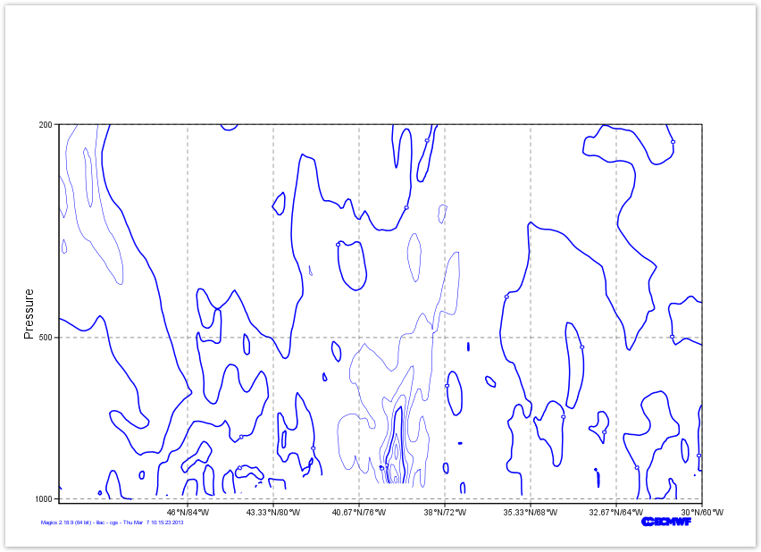
In this exercise, we want to visualise a matrix stored in a Netdef Netcdf file. Netcdf is a very generic format, and can contain a lot of data. The user needs to set up some information in order to explain to Magics which variable to plot, and how to interpret it.

...

Section

Column

width	50%

Info

title	Parameters to check

Useful Netcdf parameters
netcdf_filename
netcdf_value_variable
netcdf_field_scaling_factor
netcdf_y_variable
netcdf_x_variable
netcdf_x_auxiliary_variable

Code Block

theme	Confluence
language	python
title	Python - Loading a Netcdf
collapse	true

from Magics.macro import *
#setting the output 
output = output(    
                output_formats = ['png'],
                output_name = "xsect_step3",
                output_name_first_page_number = "off"
        )
# Setting the cartesian view
projection = mmap(
        subpage_map_projection='cartesian',
        subpage_x_axis_type='geoline',
        subpage_y_axis_type='logarithmic',
        subpage_x_min_latitude=50.,
        subpage_x_max_latitude=30.,
        subpage_x_min_longitude=-90.,
        subpage_x_max_longitude=-60.,
        subpage_y_min=1020.,
        subpage_y_max=200.,
        )
# Vertical axis
vertical = maxis(
        axis_orientation='vertical',
        axis_grid='on',
        axis_type='logarithmic',
        axis_tick_label_height=0.4,
        axis_tick_label_colour='charcoal',
        axis_grid_colour='charcoal',
        axis_grid_thickness=1,
        axis_grid_reference_line_style='solid',
        axis_grid_reference_thickness=1,
        axis_grid_line_style='dash',
        axis_title='on',
        axis_title_text='Pressure',
        axis_title_height=0.6,
        )
# Horizontal axis
horizontal = maxis(
        axis_orientation='horizontal',
        axis_type='geoline',
        axis_tick_label_height=0.4,
        axis_tick_label_colour='charcoal',
        axis_grid='on',
        axis_grid_colour='charcoal',
        axis_grid_thickness=1,
        axis_grid_line_style='dash',
        )
# Definition of the Netcdf data and interpretation
data = mnetcdf(netcdf_filename = "section.nc",
      netcdf_value_variable = "p13820121030000000000001",
      netcdf_field_scaling_factor = 100000.,
      netcdf_y_variable = "levels",
      netcdf_x_variable = "longitude",
      netcdf_x_auxiliary_variable = "latitude"
    )
contour = mcont()
plot(output, projection, horizontal, vertical, data, contour)

Column

width	200px

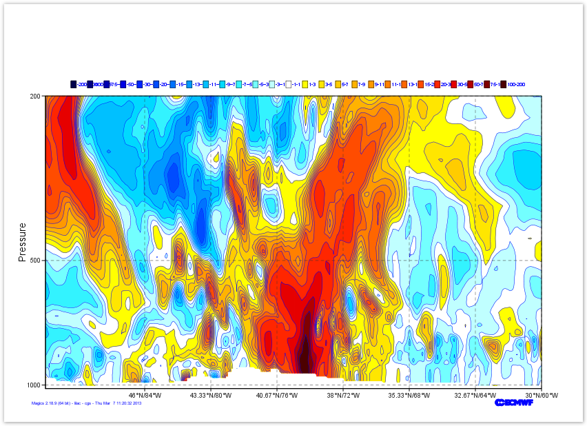
Creating a nice shading

Now, we just create a nice polygon shading.

The list of levels we want to use is : [-200., -100., -75., -50., -30., -20., -15., -13., -11., -9., -7., -5., -3., -1., 1., 3., 5., 7., 9., 11., 13., 15., 20., 30., 50., 75., 100., 200].

and the list of colours is : ["rgb(0,0,0.3)", "rgb(0,0,0.5)", "rgb(0,0,0.7)", "rgb(0,0,0.9)", "rgb(0,0.15,1)", "rgb(0,0.3,1)", "rgb(0,0.45,1)", "rgb(0,0.6,1)", "rgb(0,0.75,1)", "rgb(0,0.85,1)", "rgb(0.2,0.95,1)", "rgb(0.45,1,1)", "rgb(0.75,1,1)", "none", "rgb(1,1,0)","rgb(1,0.9,0)", "rgb(1,0.8,0)", "rgb(1,0.7,0)", "rgb(1,0.6,0)", "rgb(1,0.5,0)", "rgb(1,0.4,0)", "rgb(1,0.3,0)", "rgb(1,0.15,0)", "rgb(0.9,0,0)", "rgb(0.7,0,0)", "rgb(0.5,0,0)", "rgb(0.3,0,0)"],

Do not forget to trun the legend on ...

You could quickly check Contour Documentation

Section

Column

width	50%

Info

title	Parameters to check

Useful contour parameters
contour_level_selection_type
contour_level_list
contour_shade
contour_shade_method
contour_shade_colour_method
contour_shade_colour_list
legend

Code Block

theme	Confluence
language	python
title	Python - Using a shading
collapse	true

from Magics.macro import *
#setting the output 
output = output(    
                output_formats = ['png'],
                output_name = "xsect_step3",
                output_name_first_page_number = "off"
        )
# Setting the cartesian view
projection = mmap(
        subpage_map_projection='cartesian',
        subpage_x_axis_type='geoline',
        subpage_y_axis_type='logarithmic',
        subpage_x_min_latitude=50.,
        subpage_x_max_latitude=30.,
        subpage_x_min_longitude=-90.,
        subpage_x_max_longitude=-60.,
        subpage_y_min=1020.,
        subpage_y_max=200.,
        )
# Vertical axis
vertical = maxis(
        axis_orientation='vertical',
        axis_grid='on',
        axis_type='logarithmic',
        axis_tick_label_height=0.4,
        axis_tick_label_colour='charcoal',
        axis_grid_colour='charcoal',
        axis_grid_thickness=1,
        axis_grid_reference_line_style='solid',
        axis_grid_reference_thickness=1,
        axis_grid_line_style='dash',
        axis_title='on',
        axis_title_text='Pressure',
        axis_title_height=0.6,
        )
# Horizontal axis
horizontal = maxis(
        axis_orientation='horizontal',
        axis_type='geoline',
        axis_tick_label_height=0.4,
        axis_tick_label_colour='charcoal',
        axis_grid='on',
        axis_grid_colour='charcoal',
        axis_grid_thickness=1,
        axis_grid_line_style='dash',
        )
# Definition of the Netcdf data and interpretation
data = mnetcdf(netcdf_filename = "section.nc",
      netcdf_value_variable = "p13820121030000000000001",
      netcdf_field_scaling_factor = 100000.,
      netcdf_y_variable = "levels",
      netcdf_x_variable = "longitude",
      netcdf_x_auxiliary_variable = "latitude"
    )
contour = mcont(contour_highlight= "off",
    contour_hilo= "off",
    contour_label= "off",
    legend='on',
    contour_level_list= [-200., -100., -75., -50., -30., -20., 
        -15., -13., -11., -9., -7., -5., -3., -1., 1., 3., 5., 
        7., 9., 11., 13., 15., 20., 30., 50., 75., 100., 200],
    contour_level_selection_type= "level_list",
    contour_shade= "on",
    contour_shade_colour_list= ["rgb(0,0,0.3)", "rgb(0,0,0.5)", 
        "rgb(0,0,0.7)", "rgb(0,0,0.9)", "rgb(0,0.15,1)", 
        "rgb(0,0.3,1)", "rgb(0,0.45,1)", "rgb(0,0.6,1)", 
        "rgb(0,0.75,1)", "rgb(0,0.85,1)", "rgb(0.2,0.95,1)", 
        "rgb(0.45,1,1)", "rgb(0.75,1,1)", "none", "rgb(1,1,0)", 
        "rgb(1,0.9,0)", "rgb(1,0.8,0)", "rgb(1,0.7,0)", 
        "rgb(1,0.6,0)", "rgb(1,0.5,0)", "rgb(1,0.4,0)", 
        "rgb(1,0.3,0)", "rgb(1,0.15,0)", "rgb(0.9,0,0)", 
        "rgb(0.7,0,0)", "rgb(0.5,0,0)", "rgb(0.3,0,0)"],
    contour_shade_colour_method= "list",
    contour_shade_method= "area_fill")
plot(output, projection, horizontal, vertical, data, contour)

Column

width	200px

Image Added

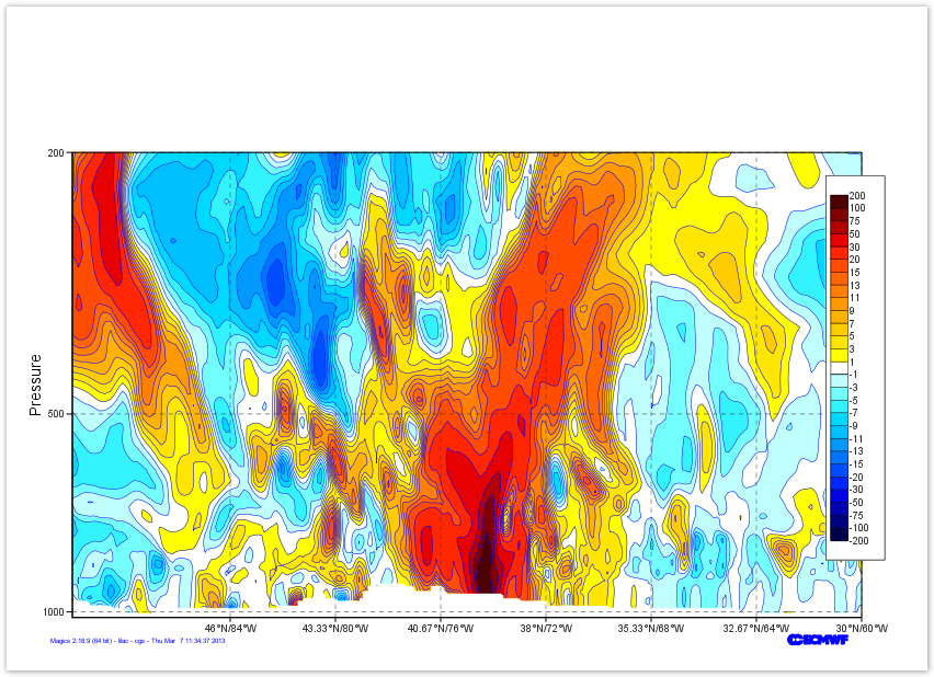
Position the legend

By default, the legend is is positioned at the top of the plot. In this exercise we want to put see our legend on a column mode on the right of the plot.

The Information about the positional mode can be found in the Legend Documentation

Column

width	50%

Info

title	Parameters to check

Useful legend parameters
legend
legend_display_type
legend_box_mode
legend_box_x_position
legend_box_y_position
legend_box_x_length
legend_box_y_length
legend_box_blanking
legend_border

Code Block

theme	Confluence
language	python
title	Python - Position the legend
collapse	true

from Magics.macro import *
#setting the output 
output = output(    
                output_formats = ['png'],
                output_name = "xsect_step5",
                output_name_first_page_number = "off"
        )
# Setting the cartesian view
projection = mmap(
        subpage_map_projection='cartesian',
        subpage_x_axis_type='geoline',
        subpage_y_axis_type='logarithmic',
        subpage_x_min_latitude=50.,
        subpage_x_max_latitude=30.,
        subpage_x_min_longitude=-90.,
        subpage_x_max_longitude=-60.,
        subpage_y_min=1020.,
        subpage_y_max=200.,
        )
# Vertical axis
vertical = maxis(
        axis_orientation='vertical',
        axis_grid='on',
        axis_type='logarithmic',
        axis_tick_label_height=0.4,
        axis_tick_label_colour='charcoal',
        axis_grid_colour='charcoal',
        axis_grid_thickness=1,
        axis_grid_reference_line_style='solid',
        axis_grid_reference_thickness=1,
        axis_grid_line_style='dash',
        axis_title='on',
        axis_title_text='Pressure',
        axis_title_height=0.6,
        )
# Horizontal axis
horizontal = maxis(
        axis_orientation='horizontal',
        axis_type='geoline',
        axis_tick_label_height=0.4,
        axis_tick_label_colour='charcoal',
        axis_grid='on',
        axis_grid_colour='charcoal',
        axis_grid_thickness=1,
        axis_grid_line_style='dash',
        )
# Definition of the Netcdf data and interpretation
data = mnetcdf(netcdf_filename = "section.nc",
      netcdf_value_variable = "p13820121030000000000001",
      netcdf_field_scaling_factor = 100000.,
      netcdf_y_variable = "levels",
      netcdf_x_variable = "longitude",
      netcdf_x_auxiliary_variable = "latitude"
    )
contour = mcont(contour_highlight= "off",
    contour_hilo= "off",
    contour_label= "off",
    legend='on',
    contour_level_list= [-200., -100., -75., -50., -30., -20., 
        -15., -13., -11., -9., -7., -5., -3., -1., 1., 3., 5., 
        7., 9., 11., 13., 15., 20., 30., 50., 75., 100., 200],
    contour_level_selection_type= "level_list",
    contour_shade= "on",
    contour_shade_colour_list= ["rgb(0,0,0.3)", "rgb(0,0,0.5)", 
        "rgb(0,0,0.7)", "rgb(0,0,0.9)", "rgb(0,0.15,1)", 
        "rgb(0,0.3,1)", "rgb(0,0.45,1)", "rgb(0,0.6,1)", 
        "rgb(0,0.75,1)", "rgb(0,0.85,1)", "rgb(0.2,0.95,1)", 
        "rgb(0.45,1,1)", "rgb(0.75,1,1)", "none", "rgb(1,1,0)", 
        "rgb(1,0.9,0)", "rgb(1,0.8,0)", "rgb(1,0.7,0)", 
        "rgb(1,0.6,0)", "rgb(1,0.5,0)", "rgb(1,0.4,0)", 
        "rgb(1,0.3,0)", "rgb(1,0.15,0)", "rgb(0.9,0,0)", 
        "rgb(0.7,0,0)", "rgb(0.5,0,0)", "rgb(0.3,0,0)"],
    contour_shade_colour_method= "list",
    contour_shade_method= "area_fill")
legend = mlegend(legend='on', 
    legend_display_type='continuous', 
    legend_text_colour='charcoal',         
    legend_text_font_size=0.4, 
    legend_box_mode = "positional",
    legend_box_x_position = 27.00,
    legend_box_y_position = 3.00,
    legend_box_x_length = 2.00,
    legend_box_y_length = 13.00,
    legend_box_blanking = "on",
    legend_border = "on",
    legend_border_colour='charcoal')
 plot(output, projection, horizontal, vertical, data, contour, legend)

Column

width	200px

Image Added

add a Title

Last thing to do here .. We add a title to the top..

Here we will use a combination of User text and automatic text ( read from the Netcdf global attribute title)

To get the automatic title, you have to use the following tag <magics_title/>

Column

width	50%

Info

title	Parameters to check

Useful legend parameters
legend
legend_display_type
legend_box_mode
legend_box_x_position
legend_box_y_position
legend_box_x_length
legend_box_y_length
legend_box_blanking
legend_border

Code Block

theme	Confluence
language	python
title	Python - Position the legend
collapse	true

from Magics.macro import *
#setting the output 
output = output(    
                output_formats = ['png'],
                output_name = "xsect_step6",
                output_name_first_page_number = "off"
        )
# Setting the cartesian view
projection = mmap(
        subpage_map_projection='cartesian',
        subpage_x_axis_type='geoline',
        subpage_y_axis_type='logarithmic',
        subpage_x_min_latitude=50.,
        subpage_x_max_latitude=30.,
        subpage_x_min_longitude=-90.,
        subpage_x_max_longitude=-60.,
        subpage_y_min=1020.,
        subpage_y_max=200.,
        )
# Vertical axis
vertical = maxis(
        axis_orientation='vertical',
        axis_grid='on',
        axis_type='logarithmic',
        axis_tick_label_height=0.4,
        axis_tick_label_colour='charcoal',
        axis_grid_colour='charcoal',
        axis_grid_thickness=1,
        axis_grid_reference_line_style='solid',
        axis_grid_reference_thickness=1,
        axis_grid_line_style='dash',
        axis_title='on',
        axis_title_text='Pressure',
        axis_title_height=0.6,
        )
# Horizontal axis
horizontal = maxis(
        axis_orientation='horizontal',
        axis_type='geoline',
        axis_tick_label_height=0.4,
        axis_tick_label_colour='charcoal',
        axis_grid='on',
        axis_grid_colour='charcoal',
        axis_grid_thickness=1,
        axis_grid_line_style='dash',
        )
# Definition of the Netcdf data and interpretation
data = mnetcdf(netcdf_filename = "section.nc",
      netcdf_value_variable = "p13820121030000000000001",
      netcdf_field_scaling_factor = 100000.,
      netcdf_y_variable = "levels",
      netcdf_x_variable = "longitude",
      netcdf_x_auxiliary_variable = "latitude"
    )
contour = mcont(contour_highlight= "off",
    contour_hilo= "off",
    contour_label= "off",
    legend='on',
    contour_level_list= [-200., -100., -75., -50., -30., -20., 
        -15., -13., -11., -9., -7., -5., -3., -1., 1., 3., 5., 
        7., 9., 11., 13., 15., 20., 30., 50., 75., 100., 200],
    contour_level_selection_type= "level_list",
    contour_shade= "on",
    contour_shade_colour_list= ["rgb(0,0,0.3)", "rgb(0,0,0.5)", 
        "rgb(0,0,0.7)", "rgb(0,0,0.9)", "rgb(0,0.15,1)", 
        "rgb(0,0.3,1)", "rgb(0,0.45,1)", "rgb(0,0.6,1)", 
        "rgb(0,0.75,1)", "rgb(0,0.85,1)", "rgb(0.2,0.95,1)", 
        "rgb(0.45,1,1)", "rgb(0.75,1,1)", "none", "rgb(1,1,0)", 
        "rgb(1,0.9,0)", "rgb(1,0.8,0)", "rgb(1,0.7,0)", 
        "rgb(1,0.6,0)", "rgb(1,0.5,0)", "rgb(1,0.4,0)", 
        "rgb(1,0.3,0)", "rgb(1,0.15,0)", "rgb(0.9,0,0)", 
        "rgb(0.7,0,0)", "rgb(0.5,0,0)", "rgb(0.3,0,0)"],
    contour_shade_colour_method= "list",
    contour_shade_method= "area_fill")
legend = mlegend(legend='on', 
    legend_display_type='continuous', 
    legend_text_colour='charcoal',         
    legend_text_font_size=0.4, 
    legend_box_mode = "positional",
    legend_box_x_position = 27.00,
    legend_box_y_position = 3.00,
    legend_box_x_length = 2.00,
    legend_box_y_length = 13.00,
    legend_box_blanking = "on",
    legend_border = "on",
    legend_border_colour='charcoal')
title = mtext(
        text_lines= ['Example of Xsection to demonstrate the use of NetCDF data...', 
        '<magics_title/>'],
        text_html= 'true',
        text_justification= 'left',
        text_font_size= 0.8,
        text_colour= 'charcoal',
        )

plot(output, projection, horizontal, vertical, data, contour, legend, title)

Image Added

Space shortcuts

Page tree

Versions Compared

Old Version 7

New Version 8

Key

Creating a nice shading

Position the legend

add a Title