Introduction
This page describes two studies of different convective cases; one over N. America associated with formation of severe tornadoes, the other over central Africa. The N.America case has strong large scale forcing whereas the central African case is driven by the diurnal cycle.
Both cases are studied starting the forecast from the same date/time (initial conditions).
In these case studies, you will carry out a control forecast, followed by any number of suggested sensitivities experiments.
US Tornado convection case (Arkansas)
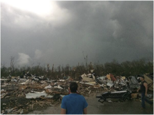
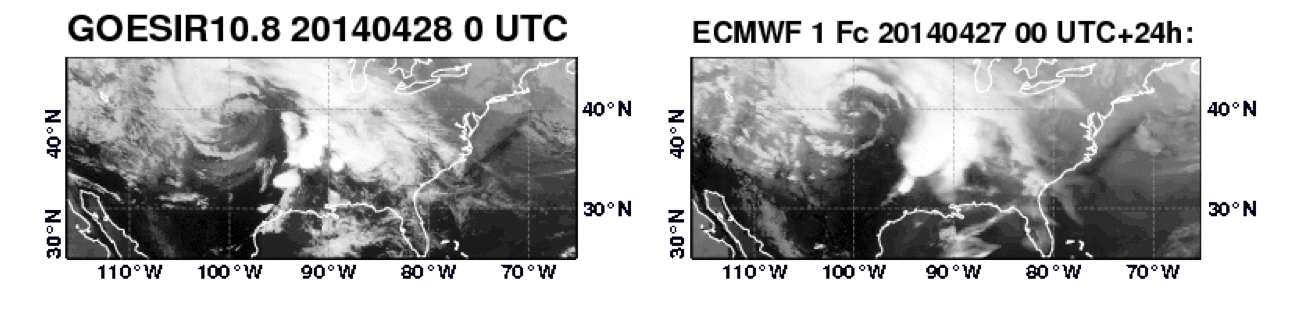
On the 27 April 7pm local time (00UTC 28 April), tornadoes hit towns north and west of Little Rock, Arkansas killing approx 17 people. (http://edition.cnn.com/2014/04/28/us/severe-weather/index.html?hpt=hp_c2). On the evening on the 28 April fatal tornadoes occurred over Mississippi (http://www.bbc.co.uk/news/world-us-canada-27199071).
This case study will look at the role of convection and the large scale in these events.
More information can also be found on the ECMWF Severe Event Catalogue 201404 - Convection - Arkansas U.S.
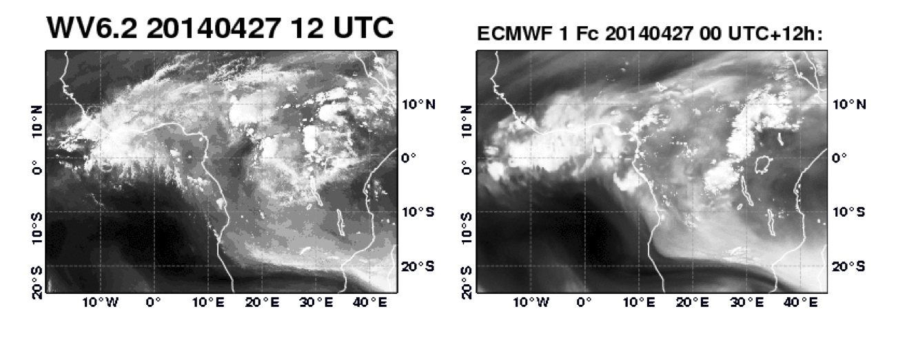
African diurnal deep convection (Central Africa)
Over tropical land masses, incoming radiation strongly heats the surface leading to the development of deep convection and precipitation. Observations show that convective activity and precipitation peak in the late afternoon or early evening. Until very recently numerical weather prediction models struggled to reproduce this diurnal cycle, often predicting convection to peak too early in the day. In this case study, aspects of the convective parameterization scheme can be altered to see how the intensity and the diurnal cycle of convection responses.
Initial conditions
Case study initial conditions for this case study are provided on the OpenIFS ftp site.
The initial conditions are available at a range of different resolutions and start dates for a 30hr forecast. The experiment ids are created at ECMWF and used for identifying the model forecasts on the ECMWF archive system (for those with access).
Note that ERA-Interim has a resolution of T255.
As OpenIFS is a spectral model, the 'T' number refers to the triangular truncation in spectral space. Equivalent grid resolutions are:
T159 ~ 125km resolution, T255 ~ 80km, T511 ~ 40km, T799 ~ 25km, T1279 ~ 16km.
TODO: table of data to download
Download instructions
% mkdir -p runs/convection/t255
% cd runs
% ftp ftp.ecmwf.int
ftp> cd case_studies/lothar_storm
ftp> binary
ftp> get 1999122412_T159_fqar.tgz
ftp> quit
% tar zxf 1999122412_T159_fqar.tgz
% ls
1999122412_T159.tgz  ICMCLfqarINIT  ICMGGfqarINIT  ICMGGfqarINIUA  ICMSHfqarINIT  ecmwf
% ls ecmwf
NODE.001_01  namelistfc
The 'ecmwf' directory contains the files produced at ECMWF when this experiment was run:
- namelistfc : copy this file to 'fort.4' to run the experiment (modify as required)
- NODE.001_01 : this is the model output file as run at ECMWF. If your run fails, it may be useful to compare with this file.
Run the control forecast
The first step is to run the control forecast. Both cases can be studied with a single forecast.
See below for tasks and key questions to address for the control forecast before moving on to the sensitivity experiments.
Case study: N.America deep convection
On 27 April 2014 7pm local time (00UTC 28 April), tornadoes hit towns north and west of Little Rock, Arkansas.

Case study: African deep convection

Sensitivity experiments
The IFS is highly tuned to give the best forecast over a range of initial conditions. However, it is instructive to try some sensitivity experiments to understand the role of various physical and dynamical processes.
Not all of the suggested experiments are applicable to both cases, indicated in brackets.
- What's the impact of the different 'lead times' on the forecast of the convection (i.e. starting from different dates)? (N.America only)
- What's the impact of resolution on the forecast of the convection? (both)
- Does reducing the model timestep improve or worsen the forecast? (both)
Turn off deep convection (both)
Impact of the improved diurnal cycle of convection. (Africa only)
In this sensitivity experiment, look at the timing of convective and precipitation events by changing how the model parametrizes the diurnal cycle.Increase the precipitation auto conversion rate - what impact does this have? (both)
Impact of the convective time scale adjustment (both)
An optimization factor in the parametrization is used for tuning the diurnal cycle. This can be altered by changing a value in the model namelist.Sensitivity to entrainment rate (both)
Additional questions
- How important is the correct diurnal cycle of precipitation and radiation for 2m temperature and dewpoint forecast?
Further reading
- P. Bechtold et al, 2014, Representing Equilibrium and Nonequilibrium Convection in Large-Scale Models. J. Atmos. Sci., 71, 734–753. http://journals.ametsoc.org/doi/abs/10.1175/JAS-D-13-0163.1
- See section on convection in description of Atmospheric Physics: http://www.ecmwf.int/en/research/modelling-and-prediction/atmospheric-physics
- More information about the N.American tornadoes can be found on the ECMWF Severe Event Catalogue - 201404 - Convection - Arkansas U.S
- ECMWF training course lecture notes on : Introduction to Moist Processes (PDF), Convection lecture 1 (PDF), Convection lecture 2 (PDF), Convection lecture 3 (PDF)
- IFS documentation, Part IV, Physical Processes - Chapter 6: convection (PDF).
- ECMWF Newsletter, summer 2014, number 140. Article on OpenIFS user workshop 2014 (Stockholm), page 2 (PDF)
Comments
The forecasting system at ECMWF makes use of "ensembles" of forecasts to account for errors in the initial state. In reality, the forecast depends on the initial state in a much more complex way than just the model resolution or starting date. At ECMWF many initial states are created for the same starting time by use of "singular vectors" and "ensemble data assimilation" techniques which change the vertical structure of the initial perturbations.
As further reading and an extension of this case study, research how these methods work.
Acknowledgements
We are grateful to: Peter Bechtold, Filip Vana, Sandor Kertesz in preparing the material for the OpenIFS user workshop in Stockholm 2014, from which most of the material on this page is derived. We also thank the forecast department for their material on the ECMWF Severe Event Catalogue that was used in preparing these cases.