Since the implementation of EFAS version 5.4 (XXX 2025) and GloFAS v4.3 (YYY 2025), the same design of products are used for the sub-seasonal range both in EFAS and GloFAS. This means, the previous EFAS sub-seasonal products were replaced by the new ones, while for GloFAS the sub-seasonal products are completely new.
The new sub-seasonal products have calendar weekly periods (i.e. always Monday-Sunday) as lead time. The forecast signal is derived from the relationship between the calendar weekly mean river discharge and the climatological distribution of the possible weekly mean values. The fixed calendar weeks, as forecast lead times, will allow the users to compare forecasts from different runs, as the verification period is fixed (as the calendar weeks). The generation of the sub-seasonal products rely on three major components, listed below:
Component-1. Real time forecasts
This part is the hydrological forecasts produced in real time. This will give the actual predicted conditions for the sub-seasonal products that will be compared to climatologies to derive the forecast anomalies. In the following we describe the characteristics of these forecast simulations. Where appropriate, the difference between EFAS and GloFAS is specified. If there is no EFAS/GloFAS mentioned, then the method is identical between the two forecast systems:
- Hydrological model: LISFLOOD (LINK!)
- Meteorological forcing: the combination of the 9km (horizontal resolution) ECMWF ensemble forecasts (LINK!) and the 36km ECMWF sub-seasonal forecasts (LINK!) from the PREVIOUS RUN
- The low-resolution sub-seasonal forcing is taken from the precious available forecast run simply because of timing, as the sub-seasonal meteo forecasts for the same day are only available with several hours delay after the high-resolution forecasts.
- The high- and low-resolution forcing is currently combined by a simple mechanical blending by using first the high resolution meteorological forcing for days 1-15, while the low-resolution meteorological forcing for days 16-45, for each of the 51 ensemble members.
- The blending can create inconsistencies locally over very complex orograpihcal areas, due to the resolution change at day15, and also there could be some smaller inconsistencies between the ensemble in the from 16 vs to 15 days, due to the mechanical blending which will mix different weather conditions from the low- and high-res meteo data, but overall as an ensemble of 51 scenarios, this will not be expected to lead to any larger discontinuities.
- Number of ensemble members: 51 ensemble members (one unperturbed and 50 perturbed) to represent the equally likely forecast scenarios of the future
- River resolution: 3arcmin (~5km) in GloFAS and 1arcmin (~1.5 km) in EFAS
- Run frequency: Forecasts are generated daily for 00 UTC
- Lead time: 45 days (1080 hours). Only 45 days, as although the low-resolution sub-seasonal meteo forecasts run out to 46 days, we can only rely on the 1-day-old run, which means we can only run the simulations to 45 days ahead
- Forecast steps: 6-hourly in EFAS and 24-hourly in GloFAS
- Forecast hydrological initialisation: From a fillup simulation forced with the shortest-range ENS-Control (unperturbed member of the ECMWF ensemble forecast) meteorological conditions
Component-2. Reforecasts
The sub-seasonal products rely on range-dependent climatologies, that change with the forecast lead time. The climatologies are produced from a large set of hydrological reforecasts. In the following we describe the characteristics of these reforecast simulations. Where appropriate, the difference between EFAS and GloFAS is specified. If there is no EFAS/GloFAS mentioned, then the method is identical between the two systems:
- Hydrological model: LISFLOOD (LINK!)
- Meteorological forcing: the combination of the 9km (horizontal resolution) ECMWF ensemble forecasts (LINK!) and the 36km ECMWF sub-seasonal forecasts (LINK!) from the SAME RUN
- The low-resolution sub-seasonal and high-resolution medium-range forcings are taken from the same forecast run date. The timing of the availability of the low-resolution forecasts is not an issue here, as these reforecasts are only produced retrospectively without any time constraints.
- The high- and low-resolution forcing is currently combined by a simple mechanical blending by using first the high resolution meteorological forcing for days 1-15, while the low-resolution meteorological forcing for days 16-46, for each of the 11 ensemble members.
- The blending can create inconsistencies locally over very complex orographical areas, due to the resolution change at day15, and also there could be some smaller inconsistencies between the ensemble in the from 16 vs to 15 days, due to the mechanical blending which will mix different weather conditions from the low- and high-res meteo data, but overall as an ensemble of 11 scenarios, this will not be expected to lead to any larger discontinuities.
- Number of ensemble members: 11 ensemble members (one unperturbed and 10 perturbed) to represent the equally likely forecast scenarios of the future
- River resolution: 3arcmin (~5km) in GloFAS and 1arcmin (~1.5 km) in EFAS
- Run frequency: Forecasts are generated always for the past 20 years. Before 12 Nov 2024, they were generated twice-weekly on Mondays and Thursdays (for 00 UTC), while from 12 Nov 2024 they are generated on given days of the months, as 1, 5, 9, 13, 17, 21, 25 and 29 (excluding 29 Feb).
- Lead time: 46 days (1104 hours)
- Forecast steps: 6-hourly in EFAS and 24-hourly in GloFAS
- Forecast hydrological initialisation: From the monitoring hydrological simulation, forced with gridded meteorological observations in EFAS and ERA5 reanalysis meteorological data in GloFAS
Component-3. Climatologies
The sub-seasonal products rely on range-dependent climatologies, that change with the forecast lead time, and which are produced from the hydrological reforecasts. The climatologies will give the reference point for the different anomaly categories applied in the sub-seasonal range. These reference points are some of the specific quantiles from the climate distribution, such as the 10th and 90th percentile values. In the following we describe the main characteristics of the climatologies. Where appropriate, the difference between EFAS and GloFAS is specified. If there is no EFAS/GloFAS mentioned, then the method is identical between the two systems:
- We currently produce climate files for each reforecast run date, so in total 8*12-1 = 95 dates in a calendar year with 1/5/9/13/17/21/25/29 of each month, excluding 29 Feb.
- For each of these climate dates, there will be climate files for each possible daily lead time of the sub-seasonal range. Here not only calendar weeks are considered, but all possible 7-day lead times, starting from days1-7, then days2-8, .., out to days 40-46 (40 possible lead times). This way, the weekly mean climatology for all possible lead times will be available, and so for each real time forecast the right climatology can be used, with the correct lead time in days, depending on which day of the week the real time forecast run (i.e. which corresponding climate lead time to choose in order to get to the calendar weeks).
- Climate sample: For the sub-seasonal, we have 20 years of reforecast with run dates roughly twice a week. For the climate sample always 3 run dates are used, the actual climate data we generate the climate for and one reforecast date before and after. For example, when generating the climate sample for 15 December 2024, all reforecasts produced for 11, 15 and 19 December will be used in the climate sample from years 2004-2023. All ensemble members are considered independently, therefore the climate sample is with 3*20*11 = 660 reforecast values for each river pixel.
- Climate distribution: The climate percentiles are produced, from 1 to 99, where the 1st percentile will the value that is exceeded 99% of the time, while the 99th percentile will be the value the reforecasts will exceed only 1% of the time. These climate percentiles will be specific to 40 possible lead times of days1-7 to days 40-46.
Generation of the forecast anomaly and uncertainty signal
In a sub-seasonal forecast, especially at the the longer ranges, the day-to-day variability of the river flow, with prediction of the actual expected flood severities, can not be predicted due to the very high uncertainties. What is possible, is to rather give an indication of the river discharge anomalies and confidence in those predicted anomalies. As the forecast range increases, the uncertainty will also generally increase and with it the sharpness of the forecast will gradually decrease and more and more often the forecast just going to show the climatologically expected conditions.
The determination of the sub-seasonal forecast signal is reflective of this and was designed to deliver a simple to understand categorical information on the anomalies and uncertainties present in the forecast, relative to the underlying climatology.
From the 660 reforecast values in the climate sample, 99 climate percentiles are determined (y-axis), which represent equally likely (1% chance) segments of the river discharge value range that occurred in the 20-year climatological sample. Figure 1 shows an example climate distribution, with only the deciles (every 10%), the two quartiles (25%, 50% and 75%), of which the middle (50%) is also called median, and few of the extreme percentiles are plotted near the minimum and maximum of the climatological range indicated by black crosses. Each of these percentiles have an equivalent river discharge value on the x-axis. From one percentile to the next, the river discharge value range is divided into 100 equally likely bins, some of which is indicated in Figure 1, such as bin1 of values below the 1st percentile, bin2 of values between the 1st and 2nd percentiles or bin 100 of river discharge values above the 99th percentiles, etc.
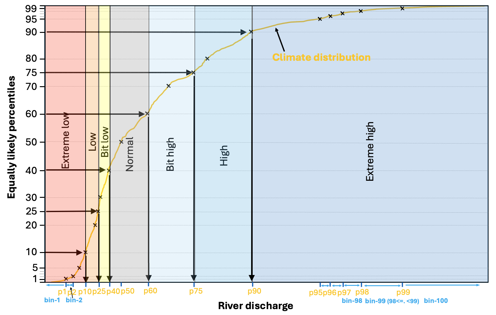
Figure 1. Schematic of the forecast anomaly categories, defined by the climatological distribution.
Based on the percentiles and the related 100 bins, there are seven anomaly categories defined. These are indicated in Figure 1 by shading. The two most extreme categories are the bottom and top 10% of the climatological distribution (<10% as red and 90%< as blue). Then the moderately low and high river discharge categories from 10-25% (orange) and 75-90% (middle-dark blue). The smallest negative and positive anomalies are defined by 25-40% and 60-75% and displayed by yellow and light blue colours in Figure 1. Finally, the normal condition category is defined from 40-60%, so the middle 1/5th of the distribution, coloured grey in Figure 1.
The forecast has 51 ensemble members, which all check where they fall in the 100 bins of the climate. This will be the anomaly or extremity value, called hereafter a rank, of the ensemble members as one of the values from 1 to 100. For example, 1 will mean the forecast value is below the 1st climate percentile (i.e. extremely anomalously low), then 2 will mean the value is between the 1st and 2nd climate percentiles (i.e. slightly less extremely low), etc., and finally 100 will mean the forecast value is above the 99th climate percentile (i.e. extremely high as higher than 99% of all the considered reforecasts representing the model climate conditions for this time of year, location and lead time).
This is possible to do for values above 0 mean river discharge, however, the rank computation becomes undefined when the values drop to 0. This is actually a major problem, as large parts of the world has dry enough areas combined with small enough catchments to have near zero or totally 0 river discharge values. For this singularity case we have a special treatment. All river discharge values below 0.1 m3/s are treated effectively as 0. All the 0 ensemble member values then get a randomly assigned rank from any of the percentiles that have 0 (i.e. below 0.1 m3/s) values in the model climatology. This effectively means, the 'rank-undefined' section of the ensemble forecast is going to be spread across the 'rank-undefined' section of the climatology during the rank computation.
Example-1:
Consider for example the following hypothetical example in Table 1. For simplicity, we represent the ensemble forecast by 21 members only (instead of 51). We also indicate below which values are considered as 0 (i.e. below 0.1 m3/s). In the 1st part of Table 1, you see the climatological percentile values, whether they are 0 or not, the possible rank values that can be assigned and the range for each of these rank values. Also, you see in the 2nd part in Table 1 the 21 ensemble member mean river discharge values, whether they are 0 or not, and then the assigned rank.
In this example, out of the 99 climate percentiles 58 are 0 (or considered 0), so this section is the undefined section where the rank computation is not directly possible. From the forecast, from the 21 represented ensemble members, 6 are (considered) 0. These 6 members will get ranks that come from the 1-58(/59) section of the 0 climatology, equally spanning it. For this example, the ranks would follow as 0, 58/5, 2*58/5, 3*58/5, 4*58/5 and finally 5*58/5, so 0, 11.6, 23.2, 34.8, 46.4 and 58. However, we can not assign fractional ranks, so we always choose the nearest integer number as rank. In this case, the ranks then would be for these 6 ensemble members: 0, 12, 23, 35, 46 and 58.
For the remaining ensemble members only few more are defined here, and the 61-96 percentiles and the related ranks are not listed here due to the limited space.
| Raw climate values | 0 | 0 | 0 | 0 | 0 | 0.01 | 0.09 | 0.11 | 0.15 | ... | 45.7 | 75.2 | 108.9 | |
| Considered as 0 (yes/no) | 1 | 1 | 1 | 1 | 1 | 1 | 1 | 0 | 0 | 0 | 0 | 0 | 0 | |
| Possible rank values | 0 | 1 | 2 | 3 | ... | 56 | 57 | 58 | 59 | 60 | ... | 97 | 98 | 99 |
| Rank description | <P1 | P1<= <P2 | P2<= <P3 | P3<= <P4 | ... | P56<= <P57 | P57<= <P58 | P58<= <P59 | P59<= <P60 | P60<= <P61 | ... | P97<= <P98 | P98<= <P99 | P99<= |
| Raw values | 0 | 0 | 0.01 | 0.05 | 0.07 | 0.09 | 0.2 | 1.4 | 3.1 | 6.3 | 9.1 | 12.1 | 14.0 | 16.0 | 18.1 | 20.1 | 24.0 | 27.1 | 30.0 | 51.1 | 109.4 |
| Considered as 0 (yes/no) | 1 | 1 | 1 | 1 | 1 | 1 | 0 | 0 | 0 | 0 | 0 | 0 | 0 | 0 | 0 | 0 | 0 | 0 | 0 | 0 | 0 |
| Ensemble member rank values | 0 | 12 | 23 | 35 | 46 | 58 | 60 | ... | ... | ... | ... | ... | ... | ... | ... | ... | ... | ... | ... | 97 | 99 |
Table 1: Hypothetic example-1 of climate distribution and the related forecast ensemble distribution represented with only 21 members.
Example-2:
In this other super extreme example (Table 2) there is no measurable river discharge in the climatology at all. this, for example can happen somewhere in the middle of the desert in the Sahara, where basically all of the daily river discharge values in the longterm reanalysis are effectively 0, and thus all the 99 percentiles of the model climatology are 0.
In the forecast, however, there are few members which have noticeable discharge, so effectively are very extreme in the climatological context, even though the absolute values are not that large necessarily. So, out of the 21 members 17 are 0 (or considered 0), and those 17 members will get ranks assigned from the 0-section of the climatology, which is in this case all the way from 0 to 99. Thus, the ranks will be as follows: 0, 99/16 (so 6 as rounded value), 2*99/16 (12), 3*99/16 (19), ..., 15*99/16 (93) and 16*99/16 (99).
Moreover, all the forecast ensemble members, which are bigger than 0.1 m3/s, will get the rank of 99 for this case with the whole climatology being below 0.1 m3/s.
| Raw climate values | 0 | 0 | 0 | 0 | 0 | 0.01 | 0.09 | |
| Considered as 0 (yes/no) | 1 | 1 | 1 | 1 | 0 | 0 | 0 | |
| Possible rank values | 0 | 1 | 2 | 3 | ... | 97 | 98 | 99 |
| Rank description | <P1 | P1<= <P2 | P2<= <P3 | P3<= <P4 | ... | P97<= <P98 | P98<= <P99 | P99<= |
| Raw values | 0 | 0 | 0 | 0 | 0 | 0 | 0 | 0 | 0 | 0 | 0 | 0 | 0 | 0 | 0 | 0.01 | 0.06 | 1.9 | 2.5 | 5 | 11 |
| Considered as 0 (yes/no) | 1 | 1 | 1 | 1 | 1 | 1 | 1 | 1 | 1 | 1 | 1 | 1 | 1 | 1 | 1 | 1 | 1 | 0 | 0 | 0 | 0 |
| Ensemble member rank values | 0 | 6 | 12 | 19 | 25 | 31 | 37 | 43 | 49 | 56 | 62 | 68 | 74 | 80 | 87 | 93 | 99 | 99 | 99 | 99 | 99 |
Table 2: Hypothetic example-2 of climate distribution and the related forecast ensemble distribution represented with only 21 members.
With this special treatment of the 0 singularity values, there is no need to mask areas on the new sub-seasonal and seasonal products. On the old version of the GloFAS seasonal forecasts, areas and time ranges, where the values were too small (effectively 0), were masked and the forecast values simply were not shown as 'undefined'.
For the new revised products, this special treatment will mean all of these 0 or near 0 cases will simply fall into an evenly distributed, very uncertain, on average near normal condition. Just as, following on from the 2nd example above, with no discharge in the climatology and no discharge in the forecast either, we will end up with a unified distribution of ranks from 0 to 99, evenly spanning the whole climatological range. Which means, if we average these ranks, we will get exactly the middle, the climate median, so no anomaly whatsoever.
This also means, for dry or very dry areas, there will never be a dry forecast anomaly, as that does not have any meaning (we can not go below 0), and therefore only neutral or positive anomalies are possible. The magnitude or severity of those positive anomalies then will be determined by the number and distribution of ensemble members being above the non-zero climate percentiles. If enough members will be above the non-zero climate percentiles and thus high enough fraction of the forecast will get high enough ranks, then on average the distribution of the 51 ensemble member ranks will show a pronounced enough shift from the neutral situation (i.e. when everything is 0 and the ranks are evenly distributed and the forecast end up looking totally normal).
- For the real time forecasts, instead we will have a 51-value ensemble of ranks (-50 to 50). So, for defining the dominant category, we have options:
- Most populated: We either choose the most populated of the 7 categories. But this will be more problematic for very uncertain cases, when little shifts in the distribution could potentially mean large shift in the categories. For example assuming a distribution of 8/7/8/7/7/7/7 and 6/7/7/7/8/9/7. These two are very much possible for the longer ranges. It is a question anyway, which one to choose in the first example, Cat1 or Cat5, they are equally likely. But then, in the 2nd case we have Cat6 as winner. But the two cases are otherwise very similar.
- ENS-mean: Alternatively, we can rather use the ensemble mean, and rank the ensemble mean value and define the severity category that way. for the above example, this would not mean a big difference, as the ensemble mean is expected to be quite similar for both forecast distributions, so the two categories will also be either the same, or maybe only one apart. I think this is what we need to do!