Download source and data
Layoutx3 Example
# Metview Macro
# **************************** LICENSE START ***********************************
#
# Copyright 2018 ECMWF. This software is distributed under the terms
# of the Apache License version 2.0. In applying this license, ECMWF does not
# waive the privileges and immunities granted to it by virtue of its status as
# an Intergovernmental Organization or submit itself to any jurisdiction.
#
# ***************************** LICENSE END ************************************
# ------------------------------------------------------------------
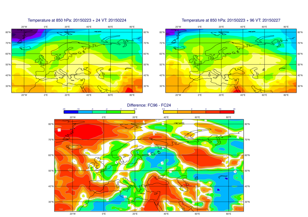
# Description: Demonstrates how to use a Display Window icon to
# produce a plot with 3 maps consisting of a) a 24h
# forecast, b) a 96h forecast and c) their difference
# ------------------------------------------------------------------
# read the GRIB data from file
t_fc24 = read(source: "t_fc24.grib", levelist: 850) # filter just the 850hPa level
t_fc96 = read(source: "t_fc96.grib", levelist: 850) # filter just the 850hPa level
# we will use the same view in all the plots, but we could also use different
# views for each plot
view = geoview(
map_area_definition : "corners",
area : [23.7,-31.6,83.0,89.6] # rough European area
)
# each page in the layout contains its position plus its view specification
# (could also be a Cross Section View, for example). Defaults are:
# top:0, bottom:100, left:0, right:100 in percent of layout height and width
page_24 = plot_page(
bottom : 45,
right : 50,
view : view
)
page_96 = plot_page(
bottom : 45,
left : 50,
view : view
)
page_diff = plot_page(
top : 50,
left : 11,
view : view
)
# contouring specifications
t_shade = mcont(
contour : "off",
contour_hilo : "off",
contour_label : "off",
contour_level_selection_type : "interval",
contour_interval : 4,
contour_shade : "on",
contour_shade_min_level : -52,
contour_shade_max_level : 48,
contour_shade_method : "area_fill",
contour_shade_colour_method : "list",
contour_shade_colour_list : ["rgb(0.88,0.2,0.88)", "rgb(0.68,0.2,0.68)", "rgb(0.48,0.2,0.48)",
"rgb(0.28,0.2,0.28)", "rgb(0.2,0,0.4)", "rgb(0.35,0,0.5)",
"blue_purple", "greenish_blue", "rgb(0,0.8,1.0)", "blue_green",
"bluish_green", "yellow_green", "greenish_yellow", "rgb(1,1,0.5)",
"yellow", "orange_yellow", "yellowish_orange", "rgb(1,0.45,0)",
"red", "rgb(0.8,0,0)", "burgundy", "rose", "magenta",
"rgb(1,0.5,1)", "rgb(1,0.75,1)"]
)
pos_shade = mcont(
legend : "on",
contour_line_colour : "grey",
contour_highlight : "off",
contour_level_selection_type : "level_list",
contour_level_list : [0.5,1,2,4,10,20],
contour_shade : "on",
contour_shade_method : "area_fill",
contour_shade_max_level_colour : "red",
contour_shade_min_level_colour : "orange_yellow",
contour_shade_colour_direction : "clockwise"
)
neg_shade = mcont(
legend : "on",
contour_line_colour : "grey",
contour_highlight : "off",
contour_level_selection_type : "level_list",
contour_level_list : [-20,-10,-4,-2,-1,-0.5],
contour_shade : "on",
contour_shade_method : "area_fill",
contour_shade_max_level_colour : "greenish_yellow",
contour_shade_min_level_colour : "blue",
contour_shade_colour_direction : "clockwise"
)
# when we have multiple pages in a layout, the default titles can be a bit too long
# for the available space; hence we will construct shorter titles, using automated
# fields as far as possible. We could also use Metview's own date/string formatting
# routines to construct 'nicer' dates in the titles
title_fc = mtext(text_line_1: "<grib_info key='name'/> at <grib_info key='level'/> hPa: "
& "<grib_info key='dataDate'/> + <grib_info key='step'/>"
& " VT: <grib_info key='validityDate'/>",
text_font_size : 0.45)
title_diff = mtext(text_line_1: "Difference: FC96 - FC24",
text_font_size : 0.45)
dw = plot_superpage(
# the order of these pages is used when indexing them in the plot() command
pages : [page_24, page_96, page_diff]
)
# define the output plot file
setoutput(pdf_output(output_name : 'layoutx3'))
# plot the data into the Cross Section view with visdefs for styling
plot(dw[1], t_fc24, t_shade, title_fc)
plot(dw[2], t_fc96, t_shade, title_fc)
plot(dw[3], t_fc96 - t_fc24, neg_shade, pos_shade, title_diff)
Layoutx3 Example
# Metview Example

#  **************************** LICENSE START ***********************************
#
#  Copyright 2018 ECMWF. This software is distributed under the terms
#  of the Apache License version 2.0. In applying this license, ECMWF does not
#  waive the privileges and immunities granted to it by virtue of its status as
#  an Intergovernmental Organization or submit itself to any jurisdiction.
#
#  ***************************** LICENSE END ************************************

# ------------------------------------------------------------------
# Description: Demonstrates how to use a Display Window icon to
#              produce a plot with 3 maps consisting of a) a 24h
#              forecast, b) a 96h forecast and c) their difference
# ------------------------------------------------------------------

import metview as mv

# read the GRIB data from file
t_fc24 = mv.read(source= "t_fc24.grib", levelist= 850) # filter just the 850hPa level
t_fc96 = mv.read(source= "t_fc96.grib", levelist= 850) # filter just the 850hPa level


# we will use the same view in all the plots, but we could also use different
# views for each plot
view = mv.geoview(
    map_area_definition = "corners",
    area                = [23.7,-31.6,83.0,89.6] # rough European area
)

# each page in the layout contains its position plus its view specification
# (could also be a Cross Section View, for example). Defaults are=
# top=0, bottom=100, left=0, right=100  in percent of layout height and width

page_24 = mv.plot_page(
    bottom = 45,
    right  = 50,
    view   = view
)

page_96 = mv.plot_page(
    bottom = 45,
    left   = 50,
    view   = view
)

page_diff = mv.plot_page(
    top    = 50,
    left   = 11,
    view   = view
)


# contouring specifications

t_shade = mv.mcont(
    contour                      = "off",
    contour_hilo                 = "off",
    contour_label                = "off",
    contour_level_selection_type = "interval",
    contour_interval             = 4,
    contour_shade                = "on",
    contour_shade_min_level      = -52,
    contour_shade_max_level      = 48,
    contour_shade_method         = "area_fill",
    contour_shade_colour_method  = "list",
    contour_shade_colour_list    = ["rgb(0.88,0.2,0.88)", "rgb(0.68,0.2,0.68)", "rgb(0.48,0.2,0.48)",
                                    "rgb(0.28,0.2,0.28)", "rgb(0.2,0,0.4)",     "rgb(0.35,0,0.5)",
                                    "blue_purple", "greenish_blue", "rgb(0,0.8,1.0)", "blue_green",
                                    "bluish_green", "yellow_green", "greenish_yellow", "rgb(1,1,0.5)",
                                    "yellow", "orange_yellow", "yellowish_orange", "rgb(1,0.45,0)",
                                    "red", "rgb(0.8,0,0)", "burgundy", "rose", "magenta",
                                    "rgb(1,0.5,1)", "rgb(1,0.75,1)"]
)

pos_shade = mv.mcont(
    legend                         = "on",
    contour_line_colour            = "grey",
    contour_highlight              = "off",
    contour_level_selection_type   = "level_list",
    contour_level_list             = [0.5,1,2,4,10,20],
    contour_shade                  = "on",
    contour_shade_method           = "area_fill",
    contour_shade_max_level_colour = "red",
    contour_shade_min_level_colour = "orange_yellow",
    contour_shade_colour_direction = "clockwise"
)

neg_shade = mv.mcont(
    legend                         = "on",
    contour_line_colour            = "grey",
    contour_highlight              = "off",
    contour_level_selection_type   = "level_list",
    contour_level_list             = [-20,-10,-4,-2,-1,-0.5],
    contour_shade                  = "on",
    contour_shade_method           = "area_fill",
    contour_shade_max_level_colour = "greenish_yellow",
    contour_shade_min_level_colour = "blue",
    contour_shade_colour_direction = "clockwise"
)


# when we have multiple pages in a layout, the default titles can be a bit too long
# for the available space; hence we will construct shorter titles, using automated
# fields as far as possible. We could also use Metview's own date/string formatting
# routines to construct 'nicer' dates in the titles

title_fc = mv.mtext(text_line_1= "<grib_info key='name'/> at <grib_info key='level'/> hPa= "
                            + "<grib_info key='dataDate'/> + <grib_info key='step'/>"
                            + " VT= <grib_info key='validityDate'/>",
                 text_font_size  = 0.45)

title_diff = mv.mtext(text_line_1= "Difference= FC96 - FC24",
                   text_font_size  = 0.45)


dw = mv.plot_superpage(
    # the order of these pages is used when indexing them in the plot() command
    pages = [page_24, page_96, page_diff]
)

# define the output plot file
mv.setoutput(mv.pdf_output(output_name = 'layoutx3'))

# plot the data into each page using a single plot command; note that
# we defined 3 pages, so they are indexed by 0, 1, 2
mv.plot(dw[0], t_fc24, t_shade, title_fc,
        dw[1], t_fc96, t_shade, title_fc,
        dw[2], t_fc96 - t_fc24, neg_shade, pos_shade, title_diff)