Page History

...

1. In general, we recommend that the hourly (analysed) "2 metre temperature" be used to construct the minimum and maximum over longer periods, such as a day, rather than using the forecast parameters "Maximum temperature at 2 metres since previous post-processing" and "Minimum temperature at 2 metres since previous post-processing".
2. ERA5: compute pressure and geopotential on model levels, geopotential height and geometric height
3. ERA5: How to calculate wind speed and wind direction from u and v components of the wind?
4. Sea surface temperature and sea-ice cover (sea ice area fraction), see Table 2 above, are available at the usual times, eg hourly for the HRES, but their content is only updated once daily.
5. Mean rates/fluxes and accumulations at step=0 have values of zero because the length of the processing period is zero.
6. Convective Inhibition (CIN). A missing value is assigned to CIN for values of CIN > 1000 or where there is no cloud base. This can occur where convective available potential energy (CAPE) is low.

7. 
   

   Expand
   title ERA5: mixing CDS and MARS data
   In the ECMWF data archive (MARS), ERA5 data is archived on various native grids. For the CDS disks, ERA5 data have been interpolated and are stored on regular latitude/longitude grids. For more information, see Spatialgrid. Storing the data on these different grids can cause incompatibilities, particularly when comparing native spherical harmonic, pressure level, MARS data with CDS disk data on a third, coarse grid. Native spherical harmonic, pressure level parameters are comprised of: Geopotential, Temperature, U component of wind, V component of wind, Vertical velocity, Vorticity, Divergence and Relative humidity. When these parameters are retrieved from MARS and a coarse output grid is specified, the default behaviour is that the spherical harmonics are truncated to prevent aliasing on the output grid. The coarser the output grid, the more severe the truncation. This truncation removes the higher wavenumbers, making the data smoother. However, the CDS disk data has been simply interpolated to the third grid, without smoothing. This incompatibility is particularly relevant when comparing ERA5.1 data (which are only available from MARS - see DataorganisationandhowtodownloadERA5 - and only for 2000-2006) with ERA5 data on the CDS disks. The simplest means of minimising such incompatibilities is to retrieve the MARS data on the same grid as that used to store the ERA5 CDS disk data.

   
   

8. 
   

   Expand
   title ERA5: Land-sea mask for wave variables
   The land-sea mask in ERA5 is an invariant field. This parameter is the proportion of land, as opposed to ocean or inland waters (lakes, reservoirs, rivers and coastal waters), in a grid box. This parameter has values ranging between zero and one and is dimensionless. In cycles of the ECMWF Integrated Forecasting System (IFS) from CY41R1 (introduced in May 2015) onwards, grid boxes where this parameter has a value above 0.5 can be comprised of a mixture of land and inland water but not ocean. Grid boxes with a value of 0.5 and below can only be comprised of a water surface. In the latter case, the lake cover is used to determine how much of the water surface is ocean or inland water.  The ERA5 land-sea mask provided is not suitable for direct use with wave parameters, as the time variability of the sea-ice cover needs to be taken into account and wave parameters are undefined for non-sea points. 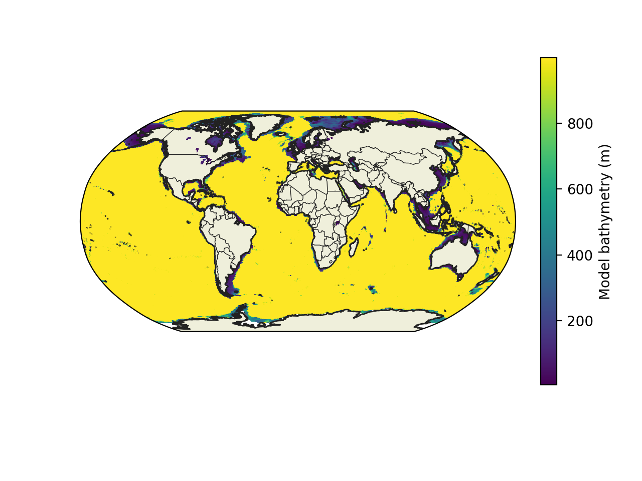In order to produce a land-sea mask for use with wave parameters, users need to download the following ERA5 data (for the required period): the model bathymetry (Model bathymetry. 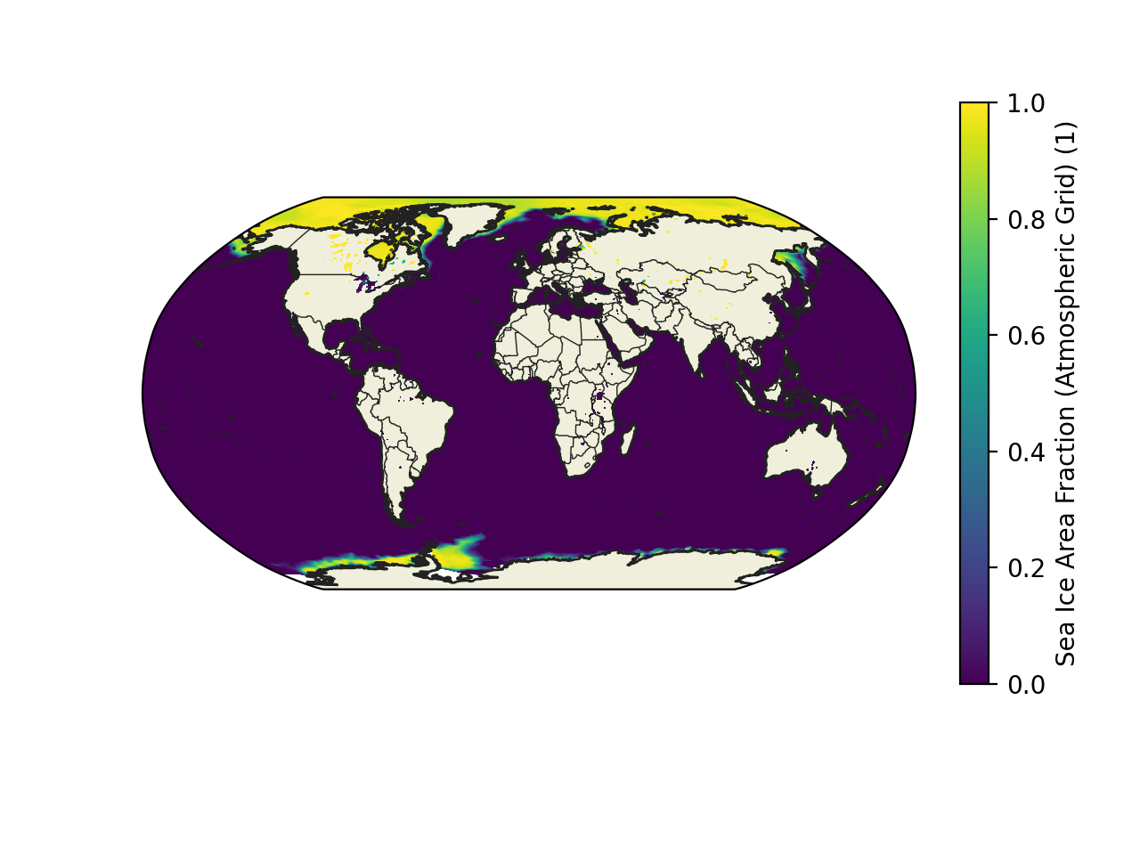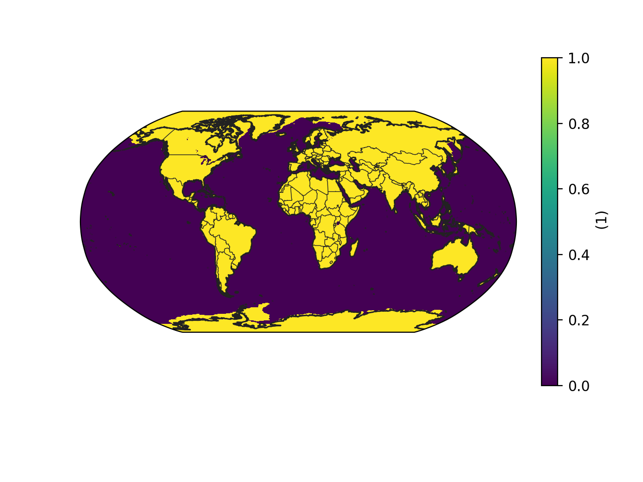Fig 1) the sea-ice cover (Sea ice area fraction, Fig 2) and combine these data to produce the land-sea mask (Fig 3). See attached pictures: Fig 1: Model bathymetry                                                 Fig 2: Sea-ice cover                                                          Fig 3: Combined mask Note Please note that sea-ice cover is only updated once daily. Please see the Toolbox workflow below to see a possible way to proceed. The results is a carousel of land-sea mask for each time step requested: Code Block title Toolbox workflow collapse true import cdstoolbox as ct @ct.application(title='Download data') @ct.output.download() @ct.output.carousel() def download_application(): count = 0 years=['1980'] months = [ '01', #'02', '03', # '04', '05', '06', # '07', '08', '09', # '10', '11', '12' ] # For hourly data hourly=True # For monthly data monthly=True hourly = True monthly = False for yr in years: for mn in months: if hourly == True: mb,si = get_hourly_data(yr, mn) elif monthly == True: mb,si = get_monthly_data(yr, mn) print(mb) # Check values are >= 0.0 in the model bathymetry mask compare_ge_mb = ct.operator.ge(mb, 0.0) print(si) # Check values are > 0.5 in the sea ice mask compare_ge_si = ct.operator.gt(si, 0.500) # Invert model bathymetry mask new = ct.operator.add(compare_ge_mb, -1.0) new1 = ct.operator.mul(new, -1.0) # Add the Bathymetry Mask to the Sea Ice Mask new_all = ct.operator.add(compare_ge_si,new1) # Reset scale to land=1, ocean=0 new_all_final = ct.operator.ge(new_all, 1.0) print(new_all_final) if count == 0: combined_mask = new_all_final else: combined_mask = ct.cube.concat([combined_mask, new_all_final], dim = 'time') count = count + 1 renamed_data = ct.cdm.rename(combined_mask, "wavemask") new_data = ct.cdm.update_attributes(renamed_data, attrs={'long_name': 'Wave Land Sea Mask'}) combined_mask = new_data print("combined_mask") print(combined_mask) # Plot mask for first timestep fig_list = ct.cdsplot.geoseries(combined_mask) return combined_mask, fig_list def get_monthly_data(y,m): m,s = ct.catalogue.retrieve( 'reanalysis-era5-single-levels-monthly-means', { 'product_type': 'monthly_averaged_reanalysis', 'variable': [ 'model_bathymetry', 'sea_ice_cover', ], 'year': y, 'month': m, 'time': '00:00', } ) return m, s def get_hourly_data(y,m): m,s = ct.catalogue.retrieve( 'reanalysis-era5-single-levels', { 'product_type': 'reanalysis', 'variable': [ 'model_bathymetry', 'sea_ice_cover', ], 'year': y, 'month': m, 'day': [ '01', '02', '03', '04', '05', '06', '07', '08', '09', '10', '11', '12', '13', '14', '15', '16', '17', '18', '19', '20', '21', '22', '23', '24', '25', '26', '27', '28', '29', '30', '31', ], 'time': [ '00:00', '01:00', '02:00', '03:00', '04:00', '05:00', '06:00', '07:00', '08:00', '09:00', '10:00', '11:00', '12:00', '13:00', '14:00', '15:00', '16:00', '17:00', '18:00', '19:00', '20:00', '21:00', '22:00', '23:00', ], } ) return m, s

   
   

9. 
   

   Expand
   title Altimeter wave parameters
   The following wave parameters are sparse observations, or quantities derived from the observations, that have been interpolated to the wave model grid and contain many missing values: altimeter_wave_height (140246) altimeter_corrected_wave_height (140247) altimeter_range_relative_correction (140248) These parameters are not available from the CDS disks but can be retrieved from MARS using the CDS API. For further guidelines, please see: Altimeter wave height in the Climate Data Store (CDS)

   
   

10. 
    

    Expand
    title Computation of near-surface humidity
    Near-surface humidity is not archived directly in ERA datasets, but the archive contains near-surface (2m from the surface) temperature (T) and dew point temperature (Td), and also surface pressure (sp), from which you can calculate specific and relative humidity at 2m. Specific humidity can be calculated using equations 7.4 and 7.5 from Part IV, Physical processes section (Chapter 7, section 7.2.1b) in the documentation of the IFS for CY41R2. Use the 2m dew point temperature and surface pressure (which is approximately equal to the pressure at 2m) in these equations. The constants in 7.4 are to be found in Chapter 12 (of Part IV: Physical processes) and the parameters in 7.5 should be set for saturation over water because the dew point temperature is being used. Relative humidity should be calculated from: RH = 100 * es(Td)/es(T)  Relative humidity can be calculated with respect to saturation over water, ice or mixed phase by defining es(T) with respect to saturation over water, ice or mixed phase (water and ice). The usual practice is to define near-surface relative humidity with respect to saturation over water. Note that in ERA5, the relative humidity on pressure levels has been calculated with respect to saturation over mixed phase.

    
    

11. 
    

    Expand
    title Computation of snow cover
    In the ECMWF model (IFS), snow is represented by an additional layer on top of the uppermost soil level. The whole grid box may not be covered in snow. The snow cover gives the fraction of the grid box that is covered in snow. For ERA5, the snow cover (SC) is computed using snow water equivalent (ie parameter SD (141.128)) as follows: Panel title ERA5 Snow cover formula snow_cover (SC) = min(1, (RW*SD/RSN) / 0.1 ) where RW is density of water equal to 1000 and RSN is density of snow (parameter 33.128). ERA5 physical depth of snow where there is snow cover is equal to RW*SD/(RSN*SC).

    
    

12. 
    

    Expand
    title Parameter "Forecast albedo" is only for diffuse radiation
    The parameter "Forecast albedo" is only for diffuse radiation and assuming a fixed spectrum of downward short-wave radiation at the surface. The true broadband, all-sky, surface albedo can be calculated from accumulated parameters: (SSRD-SSR)/SSRD where SSRD is parameter 169.128 and SSR is 176.128. This true surface albedo cannot be calculated at night when SSRD is zero. For more information, see Radiation quantities in the ECMWF model and MARS.

    
    

13. 
    

    Expand
    title Actual and potential evapotranspiration
    Actual evapotranspiration in the ERA5 single levels datasets is called "Evaporation" (param ID 182) and is the sum of the following four evaporation components (which are not available separately in ERA5 but only for ERA5-Land): Evaporation from bare soil Evaporation from open water surfaces excluding oceans Evaporation from the top of canopy Evaporation from vegetation transpiration For the ERA5 single levels datasets, actual evapotranspiration can be downloaded from the C3S Climate Data Store (CDS) under the category heading "Evaporation and Runoff", in the "Download data" tab. For details about the computation of actual evapotranspiration, please see Chapter 8 of Part IV : Physical processes, of the IFS documentation: ERA5 IFS cycle 41r2 The potential evapotranspiration in the ERA5 single levels CDS dataset is given by the parameter potential evaporation (pev).  Pev data can be downloaded from the CDS under the category heading "Evaporation and Runoff", in the "Download data" tab for the ERA5 single levels datasets. Note The definitions of potential and reference evapotranspiration may vary according to the scientific application and can have the same definition in some cases. Users should therefore ensure that the definition of this parameter is suitable for their application. Note Please note that based on ERA5 atmospheric forcing, other independent (offline) methods such us "Priesley-Taylor1 (1972) , Schmidt2 (1915) or de Bruin3 (2000)" can also be used to estimate Potential evapotranspiration. 1PRIESTLEY, C. H. B., & TAYLOR, R. J. (1972). On the Assessment of Surface Heat Flux and Evaporation Using Large-Scale Parameters, Monthly Weather Review, 100(2), 81-92. Retrieved Aug 27, 2021, from https://journals.ametsoc.org/view/journals/mwre/100/2/1520-0493_1972_100_0081_otaosh_2_3_co_2.xml  2Schmidt, W., 1915: Strahlung und Verdunstung an freien Wasserflächen; ein Beitrag zum Wärmehaushalt des Weltmeers und zum Wasserhaushalt der Erde (Radiation and evaporation over open water surfaces; a contribution to the heat budget of the world ocean and to the water budget of the earth). Ann. Hydro. Maritimen Meteor., 43, 111–124, 169–178. 3de Bruin, H. A. R., , and Stricker J. N. M. , 2000: Evaporation of grass under non-restricted soil moisture conditions. Hydrol. Sci. J., 45, 391–406, doi:10.1080/02626660009492337.

    
    

...