...
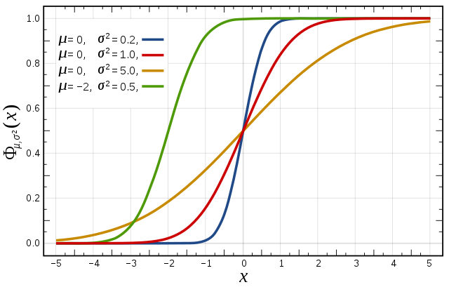
Cumulative distribution function (CDF) The figures to the right illustrate the relationship between a normal distribution and its associated cumulative distribution function.The CDF is constructed from the area under the probability density function. The CDF gives the probability that a value on the curve will be found to have a value less than or equal to the corresponding value on the x-axis. For example, in the figure right, the probability for values less than or equal to X=0 is 50%. The shape of the CDF curve is related to the shape of the normal distribution. The width of the CDF curve is directly related to the value of the standard deviation of the probability distribution function. For our ensemble, the width is then related to the 'ensemble spread'. For a forecast ensemble where all values were the same, the CDF would be a vertical straight line. |
The probability distribution function of the normal distribution |
Cumulative distribution function for a normal Figure from Wikipedia
|

...
CDF for 3 locations
This exercise uses the cdf.mv icon. Right-click, select 'Edit' and then:
...
To further understand the impact of the different types of uncertainty (initial and model), some forecasts with OpenIFS have been made in which the uncertainty has been selectively disabled. These experiments use a 40 member ensemble and are at T319 resolution, lower than the operational ensemble.
As part of this exercise you may have run OpenIFS yourself in the class to generate another ensemble; one participant per ensemble member.
Experiments available:
- EDA+SV+SPPT+SKEB SKEB : Includes initial data (EDA, SV) and model uncertainty (SPPT, SKEB) (experiment id : ens_both)
- EDA+SV only : Includes only initial data uncertainty (experiment id: ens_initial)
- SPPT+SKEB only : Includes model uncertainty only (experiment id: ens_model)
- SPPT+SKEB only, class ensemble : this is the result of the previous task using the ensemble run by the class (experiment id: oifs)
...
The aim of this exercise is to use the same visualisation and investigation to understand the impact the different types of uncertainty make on the forecast.
Follow the same tasks as above.
Plots:
as above
...
.
...
...
Task 1.
Objective: Understand the impact of changing the ensemble uncertainty
...
- Plot PV at 330K. What are the differences between the forecast? Upper tropospheric differences played a role in the development of this shallow fast moving cyclone.
extra notes
Plots:
- as above
- 4 frame: fc-an, fc-fc, pert.fc, ctl-an? *(compare the fc-fc maps with fc-an maps - can we see the uncertainty in the difference?)
- PV maps
Further reading
For more information on the stochastic physics scheme in (Open)IFS, see the article:
...