...
The generation of the sub-seasonal and seasonal forecast signal relies on few major steps. The process is illustrated by a flowchart in Figure 1. The forecast anomaly and uncertainty signal is derived by comparing the real time forecast (top left section in Figure 1) to the 99-value model climate percentiles. The climatology is generated using reforecast over a 20-year period, which provides range-dependent climate percentiles that change with the lead time. The climate generation is described in Figure 1 in the bottom right corner. Further details of the real time forecast, reforecast and the generation of the climatologies are available on this page: Placeholder Description of the real time forecasts, reforecasts and climatologies as components of the CEMS-flood sub-seasonal and seasonal forecasts.
The revised sub-seasonal products cover calendar week periods (i.e. always Monday-Sunday), while the seasonal products are valid for whole calendar month periods. The forecast signal is derived from the relationship between the calendar weekly or monthly averaged river discharge and the climatological distribution of the same weekly- or monthly-averaged values. While this naturally works for the calendar months, the fixed calendar week lead times in the sub-seasonal allow the users to directly compare forecasts from different forecast runs, as the verification period is fixed onto the calendar weeks. This way, the evolution of the subsequent daily sub-seasonal forecast runs (always at 00 UTC) can be monitored by looking at the exact same verification period.
The following step in generating anomaly and uncertainty signals is to determinesignal is determined by comparing the real time forecast ensemble members to the model climatology. This identifies, how extreme the those ensemble members of the forecast are in the context of the climatological behaviour, which is represented by the 99 percentiles and the corresponding 100 equally likely bins of the climate climatological range. This is done by ranking each ensemble member and Each ensemble member gets a rank from 1 to 100, by sorting them into one of the 100 climatological bins. This gives The real time ensemble forecast then will have 51 ranks , that range from 1 to 100.In In order to display the information content of the these 51 ensemble rank values, which all have either the calendar-weekly- or calendar-monthly-mean river discharge values or the 51 climatological ranks, a simplification was necessary. For this, 7 anomaly categories were defined from , a simplified anomaly representation was necessary. For this, 7 anomaly categories were defined by the 10th, 25th, 40th, 60th, 75th and 90th percentiles. These will span 7 categories from 'Extreme low' to 'Extreme high'. Naturally, each of these 7 categories have a probability value, depending on how many of the 51 ensemble members they contain. Moreover, the overall anomaly of the forecast is defined by the mean of the 51 ensemble member ranks (Rank-mean), which will provide a robust anomaly value no or vary minimal random jumpiness. In addition, the uncertainty about these anomalies is also defined by the 51 ensemble ranks, namely by their standard deviation (Rank-std). Based on this rank standard deviation value, one of three uncertainty categories (low / medium / high) will be assigned to the forecasts.
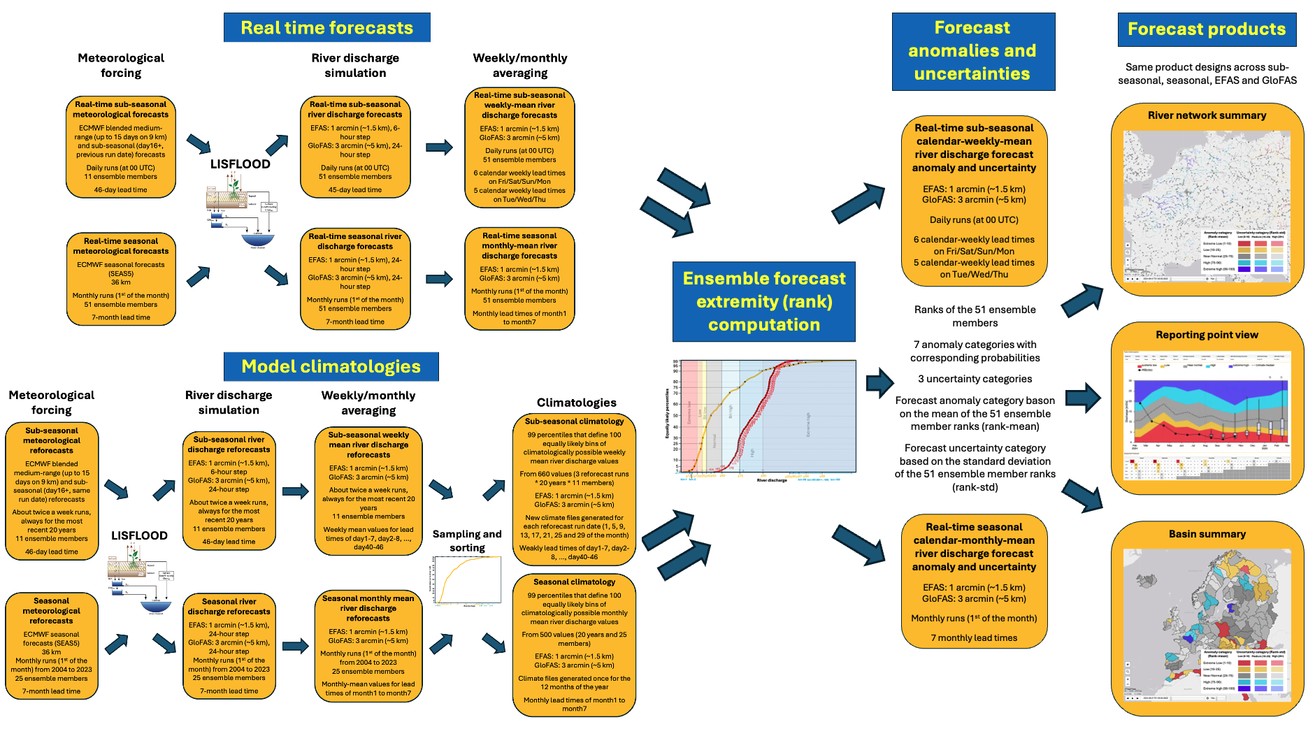
Figure 1. Flowchart of the sub-seasonal and seasonal anomaly and uncertainty signal generation methodology.
...