Since the implementation of EFAS version 5.4 and GloFAS v4.3 in 2025, the same design of products are used for both the sub-seasonal and seasonal range forecasts in EFAS and GloFAS. This means, the previous EFAS/GloFAS seasonal products and the EFAS sub-seasonal product were replaced by the new ones, while for GloFAS the sub-seasonal product was newly introduced.
The generation of the sub-seasonal and seasonal forecast signal relies on few major steps. The process is illustrated by a flowchart in Figure 1. The forecast anomaly and uncertainty signal is derived by comparing the real time forecast (top left section in Figure 1) to the 99-value model climate percentiles. The climatology is generated using reforecast over a 20-year period, which provides range-dependent climate percentiles that change with the lead time. The climate generation is described in Figure 1 in the bottom right corner. Further details of the real time forecast, reforecast and the generation of the climatologies are available on this page:
The revised sub-seasonal products cover calendar week periods (i.e. always Monday-Sunday), while the seasonal products are valid for whole calendar month periods. The forecast signal is derived from the relationship between the calendar weekly or monthly averaged river discharge and the climatological distribution of the same weekly- or monthly-averaged values. While this naturally works for the calendar months, the fixed calendar week lead times in the sub-seasonal allow the users to directly compare forecasts from different forecast runs, as the verification period is fixed onto the calendar weeks. This way, the evolution of the subsequent daily sub-seasonal forecast runs (always at 00 UTC) can be monitored by looking at the exact same verification period.
The following step in generating anomaly and uncertainty signals is to determine, how extreme the ensemble members of the forecast are in the context of the climatological behaviour, which is represented by the 99 percentiles and the corresponding 100 equally likely bins of the climate range. This is done by ranking each ensemble member and sorting them into one of the 100 climatological bins. This gives 51 ranks, that range from 1 to 100.
In order to display the information of the 51 ensemble values, which all have either the calendar-weekly- or calendar-monthly-mean river discharge values or the 51 climatological ranks, a simplification was necessary. For this, 7 anomaly categories were defined from
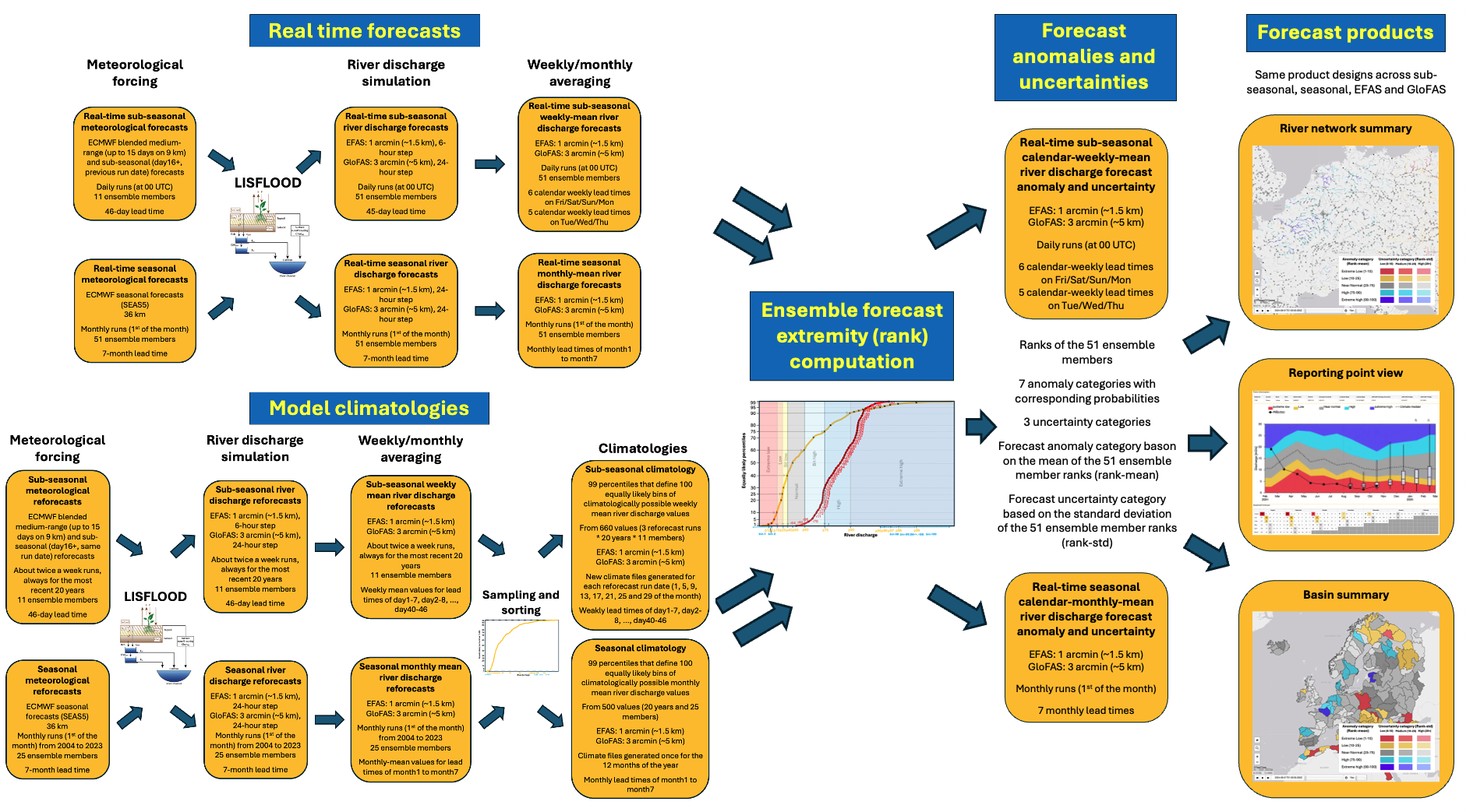
Figure 1. Flowchart of the sub-seasonal and seasonal anomaly and uncertainty signal generation methodology.
The generation of the sub-seasonal and seasonal forecast signal relies on few major steps. The process is illustrated by a flowchart in Figure 1.
Generation of the forecast anomaly and uncertainty signal
In a sub-seasonal forecast, especially at the the longer ranges, the day-to-day variability of the river flow, with prediction of the actual expected flood severities, can not be expected due to the very high uncertainties. What is possible, is to rather give an indication of the river discharge anomalies and confidence in those predicted anomalies. As the forecast range increases, the uncertainty will also generally increase and with it the sharpness of the forecast will gradually decrease and more and more often the forecast is just going to show the climatologically expected conditions with some possible positive or negative shift.
The generation of the sub-seasonal forecast signal is reflective of this and was designed to deliver a simple to understand categorical information on the anomalies and uncertainties present in the forecast, relative to the underlying weekly-mean-discharge-based climatology. The methodology to compute the anomaly and uncertainty information for the weekly mean sub-seasonal ensemble forecast is described on the page below. This page is generic and describes the procedure for any river pixel and for both the sub-seasonal and seasonal systems.
Sub-seasonal prodcuts
There are two sub-seasonal layers available on the EFAS and GloFAS websites, listed below:
Product no-1: Seasonal outlook
This product highlights the forecast signal on the rivers, including all river pixels above 50 km2 in EFAS and above 250 km2 in GloFAS. The forecast signal is indicated by colouring. The colours represent the forecast anomaly and uncertainty categories, with 5 anomaly and 3 uncertainty sub-categories, in total with 15 different types of forecast signal. Each (large enough area) river pixel will be coloured all the time, as there is always a forecast signal, even a no signal (i.e. perfectly normal condition) is going to be indicated.
Each forecast lead time is going to be individually plotted in the layer, with the control panel allowing the option to navigate/animate, the users being able to go back and force within the forecast horizon and check each forecast weekly lead time.
Details about the layer can be found in the generic description of the river network summary layer for both the sub-seasonal and seasonal, as the structure and most features are the same across the two systems here: Placeholder sub-seasonal and seasonal forecast products
Product no-2: Seasonal outlook - basins
fefwef
fw