...
- In NORMAL mode, a group of trajectories is specified starting from the same point but at different times. Several starting points (thus several groups of trajectories) can be defined for a single FLEXTRA run.
- In CET mode, trajectories are generated starting from the points of a user-defined uniform grid in a three-dimensional domain.
- In FLIGHT mode, both the starting location and starting time for each trajectory can be set individually. This mode is useful to calculate e.g. trajectories along the flight track of an aircraft.
| Info |
|---|
FLEXTRA is a free software system released under the GNU General Public License V3.0. The joint homepage of FLEXTRA and FLEXPART (a Lagrangian particle dispersion model) is hosted by the Norwegian Institute for Air Research (NILU) and available at the following address: |
| Warning |
|---|
Please note that FLEXTRA is not an ECMWF development. FLEXTRA is not distributed with Metview, but it has to be downloaded from the web site specified above and installed separately. It is installed at ECMWF though. |
...
Metview provides a high level interface to prepare input data for FLEXTRA, run FLEXTRA and visualise the resulting output files. The interface was developed and tested with version 5.0 of FLEXTRA, which is using GRIB API to handle GRIB2 fields.
The input file generation and visualisation do not require the existence of a FLEXTRA executable. However, FLEXTRA itself can be only run if an executable is present. The path to the FLEXTRA executable can be specified for Metview at installation time by setting the --with-flextra switch for configure. However, this path can be overridden at Metview start-up via the MV_FLEXTRA_EXE environment variable.
FLEXTRA is controlled through a set of parameter files which are all generated automatically by Metview in the background. The only exception is file AVAILABLE which can optionally be provided by the users (see Part 3 for details).
...
...
The Input Data
The input data needed to run the examples of this tutorial is already prepared for you and located in the directory as follows:
| Code Block |
|---|
/scratch/graphics/cgr/flextra_data |
This directory contains a set of GRIB files starting with the string "EN". These files are valid for the period of 2012-01-11 00 UTC to 2012-01-15 00 UTC. There is the AVAILABLE file here as well. It is a parameter file telling FLEXTRA the names and dates of the input GRIB files.
This dataset was generated through the Metview FLEXTRA interface. Appendix A explains how it works and helps prepare your own dataset if it is needed.
...
...
Running FLEXTRA
In this exercise we will see how to compute trajectories with FLEXTRA in NORMAL run mode. In NORMAL mode we can generate a group of trajectories starting from the same point but at different times. Please open folder 'normal' inside folder 'flextra_tutorial' to start the work.
...
To compute trajectories with FLEXTRA we need to use the FLEXTRA Run icon (right-click in the desktop when no icons are selected and use the New icon ... menu).
![]()
Rename . You can find this icon in the Modules (Data) icon drawer.
![]()
Create a new FLEXTRA Run icon by dragging it into your folder and rename it 'run_normal' and open up its editor.
First, open its editor and set the input data parameters:
...
The selected option ('Path') for parameter Flextra Input Mode indicates that we want to specify the input data and the AVAILABLE file by their paths. Because the AVAILABLE file is also located in the same directory as the input data we simply set parameter Flextra Available File Path to SAME_AS_INPUT_PATH (it is the default value). Otherwise the full path to the AVAILABLE file should have been typed in.
In the next step we will specify the starting dates of the group of trajectories we want to generate:
...
Here we set the run mode to 'NORMAL' and defined a set of forward trajectories starting on 11 January 2012 at 3, 9,12 and 15 UTC. We set the length of the trajectories to 72 h and specified that the output data (i.e. trajectory waypoints) will be written out every three hours.
The last step is
| Warning | ||
|---|---|---|
| ||
FLEXTRA cannot start the computations from the very first available date and time. So we could start from 2012-01-11 00 UTC (the first available date and time in our data) as a starting date and time but had to use the next step (3h). |
The last step is to define the starting point parameters:
...
With these settings we specified the trajectory type to be three-dimensional (see below for the list of IDs for trajectory types) and set the starting point to volcano Katla (on Iceland) with the height of 1512m.
Please note that if global GRIB2 input fields generated by Metview are used in FLEXTRA 5 it incorrectly detects the domain and treats it as a limited area. As a consequence trajectories cannot cross the domain boundaries because the computation stops at the border.
Another problem with such input fields is that FLEXTRA thinks that the longitude span of the domain is either 0-360 degrees or 180-540 (!!!) degrees depending on the geometry settings in the GRIB headers (the actual range can be figured out from the header of the result files FLEXTRA produces). In both cases we need to guarantee that the starting point we specify is in the given coordinate range. Otherwise FLEXTRA fails with the following message:
"NOTICE: STARTING POINT OUT OF DOMAIN HAS BEEN DETECTED"
In the first case it is trivial to ensure it, while in the second case we need to add 360 to the longitude to make FLEXTRA accept the starting point.
We would like to emphasise again that it happens only to global fields and only if these are encoded in GRIB2.
Remarks
- Please note that FLEXTRA cannot start the computations from the very first available date and time. So we could not use 2012-01-11 00 UTC (the first date and time in our data) as a starting date and time.
- The format of parameters holding dates is yyyymmdd. Any dates having less than 8 digits are interpreted as relative dates. E.g, -1 = yesterday, 0 = today, 1 = tomorrow etc.
- The format of parameters holdings times is hh:mm:ss with the following rules:
- If mm:ss is omitted it defaults to hh (without the colon!). E,g. 12 = 12 h
- The leading zero is not mandatory for hh. E.g.: 2 = 2 h
- If ss is omitted it defaults to hh:mm. E.g. 12:30 = 12 h 30 m
- Parameters Flextra Trajectory Length, Flextra Starting Time Interval and Flextra Output Interval Value have the format of hhh:mm:ss. The following rules apply:
- If ss is omitted it defaults to hhh:mm. E.g. "120:30" = 120 h 30 m 0 s
- If mm:ss is omitted it defaults to hhh. E.g. 120 = 120 h
- The leading zero is not mandatory for hhh. E.g.: 12 = 12 h
- We set the trajectory type by its ID. The possible values are as follows:
- Three-dimensional
- Model layer
- Mixing layer
- Isobaric
- Isentropic
- The level units were also given by an ID. The possible values are as follows:
- Metres above sea level
- Metres above ground level
- Hectopascals
- Parameter Flextra Output Interval Mode controls how the trajectory points are written out into the output file. It can have three values:
- Original: The trajectory points are written out into the output file exactly at the computational time steps. In the FLEXTRA terminology these are called flexible time steps.
- Interval: The trajectory points are written out into the output file at regular intervals specified by parameter Flextra Output Interval Value. In the FLEXTRA terminology these are called constant time steps.
- Both: Two output files will be generated: one for the flexible time steps and one for the constant time steps (in Part 11 we will see how to deal with multiple FLEXTRA outputs).
- We only specified one starting point but in Part 11 we will see how to work with multiple starting points for a NORMAL run.
Remarks
The format of parameters holding dates is yyyymmdd. Any dates having less than 8 digits are interpreted as relative dates. E.g, -1 = yesterday, 0 = today, 1 = tomorrow etc.
The format of parameters holdings times is hh:mm:ss with the following rules:
- If mm:ss is omitted it defaults to hh (without the colon!). E,g. 12 = 12 h
- The leading zero is not mandatory for hh. E.g.: 2 = 2 h
- If ss is omitted it defaults to hh:mm. E.g. 12:30 = 12 h 30 m
Parameters Flextra Trajectory Length, Flextra Starting Time Interval and Flextra Output Interval Value have the format of hhh:mm:ss. The following rules apply:
- If ss is omitted it defaults to hhh:mm. E.g. "120:30" = 120 h 30 m 0 s
- If mm:ss is omitted it defaults to hhh. E.g. 120 = 120 h
- The leading zero is not mandatory for hhh. E.g.: 12 = 12 h
We set the trajectory type by its ID. The possible values are as follows:
- Three-dimensional
- Model layer
- Mixing layer
- Isobaric
- Isentropic
The level units were also given by an ID. The possible values are as follows:
- Metres above sea level
- Metres above ground leve
- Hectopascals
Parameter Flextra Output Interval Mode controls how the trajectory points are written out into the output file. It can have three values:
- Original: The trajectory points are written out into the output file exactly at the computational time steps. In the FLEXTRA terminology these are called flexible time steps.
- Interval: The trajectory points are written out into the output file at regular intervals specified by parameter Flextra Output Interval Value. In the FLEXTRA terminology these are called constant time steps.
- Both: Two output files will be generated: one for the flexible time steps and one for the constant time steps (in Part 11 we will see how to deal with multiple FLEXTRA outputs).
We only specified one starting point but in Part 11 we will see how to work with multiple starting points for a NORMAL run.
| Note | ||
|---|---|---|
| ||
If global GRIB2 input fields generated by Metview are used in FLEXTRA 5 it incorrectly detects the domain and treats it as a limited area. As a consequence trajectories cannot cross the domain boundaries because the computation stops at the border. |
| Note | ||
|---|---|---|
| ||
Another problem with global GRIB2 input fields is that FLEXTRA interprets the longitude span of the domain either as 0-360 or 180-540 (!!!) degrees depending on the geometry settings in the GRIB headers. The actual range can be figured out from the header of the FLEXTRA output files. In both cases we need to guarantee that the starting point we specify is in the given coordinate range. Otherwise FLEXTRA fails with the following message:
In the first case it is trivial to ensure it, while in the second case we need to add 360 to the longitude to make FLEXTRA accept the starting point. |
Running FLEXTRA
Save your FLEXTRA Run icon (Apply) then right-click and execute to start the trajectory computations. Within a minute (it might take longer on your machine) the icon should turn green indicating that the run was successful and the results have been cached.
...
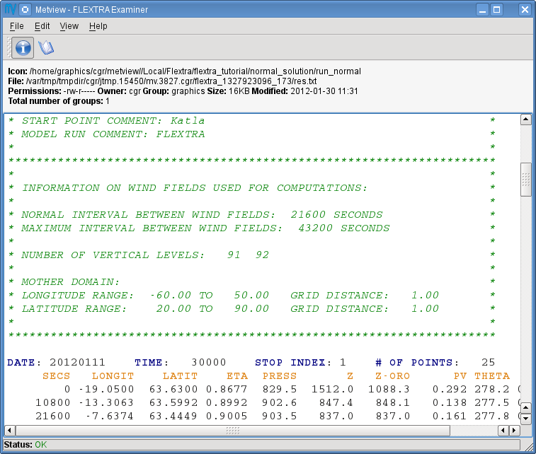
Our FLEXTRA run generated an ASCII file on output which is now represented by our FLEXTRA Run icon. Right-click and examine the icon to look to see its content. This action will start up a window showing the output generated by FLEXTRA. What you are looking at is a custom ASCII format describing the resulting trajectories and some metadata.
Now close the FLEXTRA examiner. Right-click and save the icon to get a local copy of the FLEXTRA output file. A File Save dialog will appear with a Selection box at the bottom where you can specify the output file name. Type here 'res_normal.txt' and click Ok. After a few seconds a FLEXTRA File icon with the selected name will appear in your folder.
![]()
This icon now stores your FLEXTRA output data. You can check its content by right-click and examine or edit.
Please note that saving
| Info |
|---|
Saving the results into a file is not essential for using trajectories in Metview but allows you to have a local copy of the results for further processing outside Metview. Be aware that cached data gets deleted on exiting Metview. It means that the trajectory result data stored by the FLEXTRA RUN icon will be deleted between two Metview sessions. Therefore, especially if the computations take a long time, it is worth saving the results into a file. |
Remarks
Flextra assigns an exit code called stop index for each trajectory. Its value can be seen in the FLEXTRA output (the examiner highlights it in blue in the trajectory header). The possible values are as follows:
...
- Normal exit.
- The trajectory left the computation domain.
- The time difference between two wind fields was too large.
- No wind fields were available.
...
...
Visualisation On Maps
In this exercise we will visualise the trajectories that we computed in the previous chapter. We will work in folder 'normal' again.
...
To visualise your FLEXTRA output you need to use a FLEXTRA Visualiser icon (it can be found in the Modules (Plotting) icon drawer).
![]()
Create a new FLEXTRA Visualiser icon by dragging it into your folder and rename it 'plot_normal'. Edit it and drop your 'run_normal' FLEXTRA Run icon into the Flextra Data field. This specifies the FLEXTRA output to be visualised. (Please note that you could also have dropped your 'res_normal.txt' FLEXTRA File icon into the FLEXTRA Data field to specify the data to be plotted).
At this point we do not need to set any other parameters the default values will work for us. After these modifications your icon editor should look like this.

Visualising the Icon
Save your FLEXTRA Visualiser icon (Apply) then right-click and visualise to plot the trajectories. This will bring up the Metview Display Window using a custom visualisation assigned to FLEXTRA files.
What you are looking at is a global map (it might be different for you depending on your Map View settings) on which the trajectories are hard to see. There is a Map View icon called 'map_Katla' prepared for you in the folder and we suggest that you drop it into the plot to get the right area and a shaded map background as well (alternatively you can zoom into this area).
The first thing to note in the plot is the title. It reads as
FLEXTRA: Forward 3D 1512m Katla (-19.05,63.63)
telling us that we visualised a set of 3D forward trajectories starting from the point called 'Katla'. The legend contains the starting date, time and elevation for each trajectory.
Now click on the 'plot_normal' layer in the Layers tab (on the right hand side of the plot window). If you change the view by clicking on the View metadata toggle button
![]()
you will see the meta-data associated with the visualised trajectories.

...
Our plot was generated by using hard-coded symbol plotting settings for trajectory rendering. Now we will change these settings and learn how to customise the graphical properties of individual trajectories.
To start with, we have to be aware that Metview assigns an integer ID to each trajectory before it gets visualised. The numbering starts at 1 and the original trajectory order is kept. In this way we assign the value thevalue of 1 to all the points in the first trajectory. We assign the value of 2 to the points if the second trajectory and so on for the rest of the trajectories. Then in the visualisation Metview uses symbol plotting to assign different graphical attributes to different values i.e. for different trajectories.
To see how it is working in detail let's create a Symbol Plotting icon (it can be found in the Visual Definitions icon drawer, you may need to scroll the drawers to the right). Rename it 'symbol' then edit it. ![]()
First, we need to set the symbol plotting type:
...
- The identifiers of the available symbol markers are summarised in the table below:

- We could have specified a list of symbol heights for parameter Advanced Symbol Table Height List.
...
Visualisation on XY Plots
In this exercise we will display the temporal evolution of the height of the trajectories we computed in Part 3 . We will generate a graph plot with having the date as the horizontal axis and the height as the vertical axis. We will work in folder 'normal' again.
...
The visualisation is based on the FLEXTRA Visualiser icon just like in the case of the map-based plotting in the previous exercise (Part 4 ).
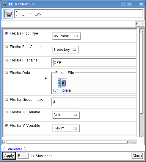
Create a new FLEXTRA Visualiser icon and rename it 'plot_normal_xy' then open its editor.
First, set Flextra Plot Type to 'Xy Points' to indicate that we want to plot symbols in a Cartesian co-ordinate system.
Second, drop your 'run_normal' FLEXTRA Run icon into the Flextra Data field. This specifies the FLEXTRA output to be visualised.
Last, we need to specify the data to be used for the x-axis and y-axis, respectively. Here we set Flextra X Variable to 'Date' and Flextra Y Variable to 'Height'.
After these modifications your icon editor should look like this.
Visualising the Icon
Save your FLEXTRA Visualiser icon (Apply) then right-click and visualise to plot the trajectories.

The Metview Display Window is popping up using a custom visualisation assigned to FLEXTRA files. The title and a legend have been built exactly in the same way as in the map-based visualisation (see Part 4 ).
...
We selected Reading as the end point and set the height to 1500 metres. We defined the trajectory type to be three-dimensional.
Running FLEXTRA
Save your FLEXTRA Run icon (Apply) then right-click and execute to start the trajectory computations. Within a minute (it might take longer on your machines) the icon should turn green indicating that the run was successful and the results have been cached. Right-click and examine the icon to look at its content. Please note that the first data column contains negative values indicating that we computed backward trajectories.

...
With these settings we defined a horizontal grid with only one point (exactly at the position of volcano Katla) and specified four vertical layers from 1500 to 3000 m above seal level.
Running FLEXTRA
Save your FLEXTRA Run icon (Apply) then right-click and execute to start the trajectory computations. Within a minute (it might take longer on your machines) the icon should turn green indicating that the run was successful and the results have been cached. Right-click and examine the icon to look at its content.
...
Here we set the trajectory mode to 'FLIGHT' and defined an imaginary flight track called 'track' with 3 points each being valid at a different time.
Running FLEXTRA
Save your FLEXTRA Run icon (Apply) then right-click and execute to start the trajectory computations. Within a minute (it might take longer on your machine) the icon should turn green indicating that the run was successful and the results have been cached. Right-click and examine the icon to look at its content.
...
Key | Description | Retrun value |
date | Date. | list of dates |
eta | Model level. | vector |
lat | Latitude. | vector |
lon | Longitude. | vector |
pres | Pressure. | vector |
pv | Potential vorticity. | vector |
startDate | Date of starting point. | string |
startEta | Model level of starting point. | string |
startLat | Latitude of starting point. | string |
startLon | Longitude of starting point. | string |
startPres | Pressure of starting point. | string |
startPv | Potential vorticity of starting point. | string |
startTheta | Potential temperature of starting point. | string |
startTime | Time of starting point. | string |
startZ | Height (above sea) of starting point | string |
startZAboveGround | Height (above ground) of starting point | string |
stopIndex | Stop index of computations. | string |
theta | Potential temperature. | vector |
z | Height above sea level. | vector |
zAboveGroundLevel | Height above ground level. | vector |
| Anchor | ||||
|---|---|---|---|---|
|
...
Here we defined two starting points: volcano Katla (as in Part 3 ) and volcano Stromboli. We set the starting heights to the real heights of these volcanoes and again we defined the trajectory types to be three-dimensional.
Running FLEXTRA
Save your FLEXTRA Run icon (Apply) then right-click and execute to start the trajectory computations. Within a minute (it might take longer on your machine) the icon should turn green indicating that the run was successful and the results have been cached.
...