...
| Note | ||
|---|---|---|
| ||
Please note that this tutorial requires Metview version 4.3.0 or later. |
| Table of Contents |
|---|
Preparations
First start Metview; at ECMWF, the command to use is metview (see Metview at ECMWF for details of Metview versions). You should see the main Metview desktop popping up.
...
Last find the newly created flextra_tutorial folder in the Metview desktop and open it (double-click to open). You should see the following contents:

Introduction
What is FLEXTRA?
FLEXTRA is an atmospheric trajectory model used by a large user community. It can be driven by meteorological input data from a variety of global and regional models including ECMWF analyses and forecasts.
...
| Warning |
|---|
Please note that FLEXTRA is not an ECMWF development. FLEXTRA is not distributed with Metview, but it has to be downloaded from the web site specified above and installed separately. It is installed at ECMWF though. |
About the Metview interface
Metview provides a high level interface to prepare input data for FLEXTRA, run FLEXTRA and visualise the resulting output files. The interface was developed and tested with version 5.0 of FLEXTRA, which is using GRIB API to handle GRIB2 fields.
...
FLEXTRA is controlled through a set of parameter files which are all generated automatically by Metview in the background. The only exception is file AVAILABLE which can optionally be provided by the users (see Part 3 for details).
The Input Data
The input data needed to run the examples of this tutorial is already prepared for you and located in the directory as follows:
...
This dataset was generated through the Metview FLEXTRA interface. Appendix A explains how it works and helps prepare your own dataset if it is needed.
Running FLEXTRA
In this exercise we will see how to compute trajectories with FLEXTRA in NORMAL run mode. In NORMAL mode we can generate a group of trajectories starting from the same point but at different times. Please open folder 'normal' inside folder 'flextra_tutorial' to start the work.
The FLEXTRA Run Icon
To compute trajectories with FLEXTRA we need to use the FLEXTRA Run icon (right-click in the desktop when no icons are selected and use the New icon ... menu).
...
With these settings we specified the trajectory type to be three-dimensional (see below for the list of IDs for trajectory types) and set the starting point to volcano Katla (on Iceland) with the height of 1512m.
Remarks
The format of parameters holding dates is yyyymmdd. Any dates having less than 8 digits are interpreted as relative dates. E.g, -1 = yesterday, 0 = today, 1 = tomorrow etc.
...
| Note | ||
|---|---|---|
| ||
Another problem with global GRIB2 input fields is that FLEXTRA interprets the longitude span of the domain either as 0-360 or 180-540 (!!!) degrees depending on the geometry settings in the GRIB headers. The actual range can be figured out from the header of the FLEXTRA output files. In both cases we need to guarantee that the starting point we specify is in the given coordinate range. Otherwise FLEXTRA fails with the following message:
In the first case it is trivial to ensure it, while in the second case we need to add 360 to the longitude to make FLEXTRA accept the starting point. |
Running FLEXTRA
Save your FLEXTRA Run icon (Apply) then right-click and execute to start the trajectory computations. Within a minute (it might take longer on your machine) the icon should turn green indicating that the run was successful and the results have been cached.
The FLEXTRA File icon
Our FLEXTRA run generated an ASCII file on output which is now represented by our FLEXTRA Run icon. Right-click and examine the icon to look to see its content. This action will start up a window showing the output generated by FLEXTRA. What you are looking at is a custom ASCII format describing the resulting trajectories and some metadata.
...
| Info |
|---|
Saving the results into a file is not essential for using trajectories in Metview but allows you to have a local copy of the results for further processing outside Metview. Be aware that cached data gets deleted on exiting Metview. It means that the trajectory result data stored by the FLEXTRA RUN icon will be deleted between two Metview sessions. Therefore, especially if the computations take a long time, it is worth saving the results into a file. |
Visualisation On Maps
In this exercise we will visualise the trajectories that we computed in the previous chapter. We will work in folder 'normal' again.
The FLEXTRA Visualiser Icon
To visualise your FLEXTRA output you need to use a FLEXTRA Visualiser icon.
...
At this point we do not need to set any other parameters the default values will work for us. After these modifications your icon editor should look like this.

Visualising the Icon
Save your FLEXTRA Visualiser icon (Apply) then right-click and visualise to plot the trajectories. This will bring up the Metview Display Window using a custom visualisation assigned to FLEXTRA files.
...
you will see the meta-data associated with the visualised trajectories.

Customising the Plot
Our plot was generated by using hard-coded symbol plotting settings for trajectory rendering. Now we will change these settings and learn how to customise the graphical properties of individual trajectories.
...
- We could have specified a list of symbol heights for parameter Advanced Symbol Table Height List.
Visualisation on XY Plots
In this exercise we will display the temporal evolution of the height of the trajectories we computed in Part 3 . We will generate a graph plot with having the date as the horizontal axis and the height as the vertical axis. We will work in folder 'normal' again.
Creating a FLEXTRA Visualiser Icon
The visualisation is based on the FLEXTRA Visualiser icon just like in the case of the map-based plotting in the previous exercise (Part 4 ).
...
After these modifications your icon editor should look like this.
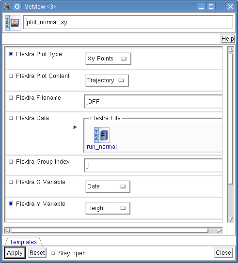
Visualising the Icon
Save your FLEXTRA Visualiser icon (Apply) then right-click and visualise to plot the trajectories.

The Metview Display Window is popping up using a custom visualisation assigned to FLEXTRA files. The title and a legend have been built exactly in the same way as in the map-based visualisation (see Part 4 ).
Customising the Plot
Our plot was generated by using hard-coded symbol plotting settings for trajectory rendering. We can change these settings exactly in the same way as we did for our map-based plot (see Part 4 for details). Now we will not create a new icon but simply reuse the Symbol Plotting icon called 'symbol' we created in Part 4 . Drop this icon into the plot to see the effect of the settings.
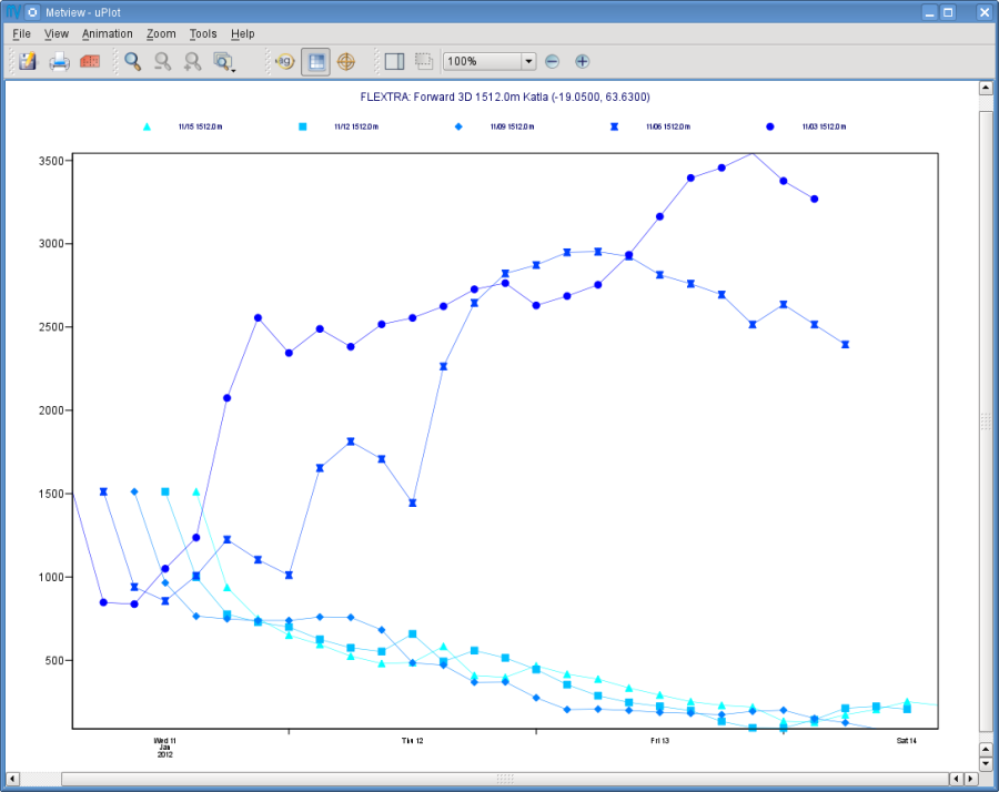
Changing the View
We will further customise the plot by changing the axis value ranges and adding axis labels and grid-lines to it. To change these properties we need a Cartesian View icon. This time you do not need to create a new icon since there is one called 'xy_view' already prepared for you. Edit his icon to see how the view is constructed (please note that the axis properties are defined via the embedded Horizontal Axis and Vertical Axis icons). Then simply drag it into the Display Window and see how you plot has been changed.

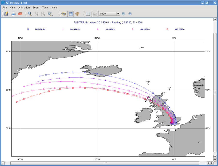
Backward Trajectories
In this exercise we will see how to compute backward trajectories with FLEXTRA in NORMAL run mode. We will work in folder 'normal' again.
Creating a FLEXTRA Run Icon
Copy your 'run_normal' FLEXTRA Run icon (either right-click + duplicate, or drag with the middle mouse button), and rename the duplicate 'run_normal_back' by clicking on its title. Open its editor and start editing the date and time related parameters (the input data parameters are already set correctly for us so we do not need to change them):
...
We selected Reading as the end point and set the height to 1500 metres. We defined the trajectory type to be three-dimensional.
Running FLEXTRA
Save your FLEXTRA Run icon (Apply) then right-click and execute to start the trajectory computations. Within a minute (it might take longer on your machines) the icon should turn green indicating that the run was successful and the results have been cached. Right-click and examine the icon to look at its content. Please note that the first data column contains negative values indicating that we computed backward trajectories.

Visualising the Results
We can visualise the results in exactly the same way as we did in the previous chapter.
Create a new FLEXTRA Visualiser icon. Edit it and drop your 'normal_run_back' FLEXTRA Run icon into the Flextra Data field. Now save your settings (Apply) then right-click and visualise to plot the trajectories. After zooming into the proper area (or dropping the map_Reading icon into the plot) you should see something like this.
CET Run Mode
In this exercise we will see how to compute trajectories with FLEXTRA in CET run mode. In this mode we can generate a set of trajectories starting from the points of a uniform three-dimensional grid. Please open folder 'cet' inside 'flextra_tutorial' to start the work.
Creating a FLEXTRA Run Icon
Create a new FLEXTRA Run icon and rename it 'run_cet' then open its editor.
...
With these settings we defined a horizontal grid with only one point (exactly at the position of volcano Katla) and specified four vertical layers from 1500 to 3000 m above seal level.
Running FLEXTRA
Save your FLEXTRA Run icon (Apply) then right-click and execute to start the trajectory computations. Within a minute (it might take longer on your machines) the icon should turn green indicating that the run was successful and the results have been cached. Right-click and examine the icon to look at its content.
Visualising the Results
We can visualise the results in exactly the same way as we did in the previous chapters.
Create a new FLEXTRA Visualiser icon. Edit it and drop your 'run_cet' FLEXTRA Run icon into the Flextra Data field. Now save your settings (Apply) then right-click and visualise to plot the trajectories. After zooming into the proper area (or dropping the map_Katla Map View icon into the plot) you should see something like this.

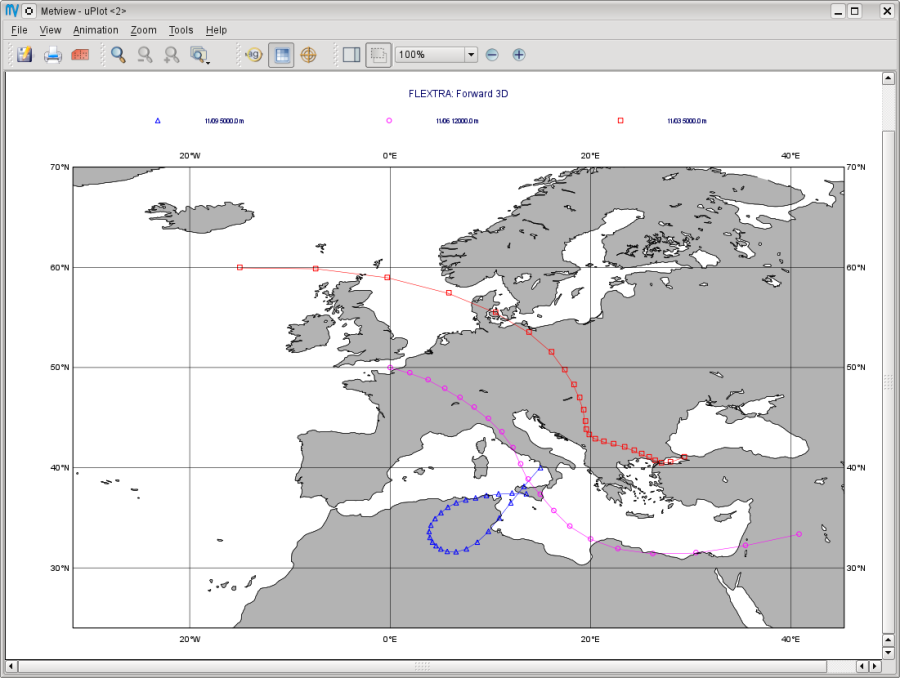
FLIGHT Run Mode
In this exercise we will see how to compute trajectories with FLEXTRA in FLIGHT run mode. In this mode, we can specify the starting location and starting time for each trajectory individually. It is useful to calculate, for instance, trajectories along the flight track of an aircraft. Please open folder 'flight' inside 'flextra_tutorial' to start the work.
Creating a FLEXTRA Run Icon
Create a new FLEXTRA Run icon and rename it 'run_flight' then open its editor.
First, we need to set the input data parameters (in the same way as we did it in Part 3 ):
...
Here we set the trajectory mode to 'FLIGHT' and defined an imaginary flight track called 'track' with 3 points each being valid at a different time.
Running FLEXTRA
Save your FLEXTRA Run icon (Apply) then right-click and execute to start the trajectory computations. Within a minute (it might take longer on your machine) the icon should turn green indicating that the run was successful and the results have been cached. Right-click and examine the icon to look at its content.
Visualising the Results
We can visualise the results in exactly the same way as we did in the previous chapter.
Create a new FLEXTRA Visualiser icon. Edit it and drop your 'run_flight' FLEXTRA Run icon into the Flextra Data field. Now save your settings (Apply) then right-click and visualise to plot the trajectories. After zooming into the proper area (or dropping the map_Eu icon Map View into the plot) you should see something like this.
Using Macro
In this example we will write the macro equivalent of the exercise we solved in Part 3 and Part 4 : we will compute forward trajectories with FLEXTRA in the NORMAL run mode and then visualise them. Please open folder 'normal' inside 'flextra_tutorial' to start the work.
Basics
The implementation of FLEXTRA-related operations in Metview macro follow the same principles as in the interactive mode. In macro we work with the macro command equivalents of the FLEXTRA icons we have seen so far:
...
There is also a macro equivalent command for icon FLEXTRA Prepare, which is used to prepare input data for FLEXTRA. Please see Appendix A for details on it.
Automatic macro generation
The quickest way to generate a macro is to simply save a visualisation on screen as a Macro icon. Visualise your 'plot_normal' FLEXTRA Visualiser icon again and click on the macro icon in the tool bar of the Display Window.

Now a new Macro icon called 'MacroFrameworkN' is generated in your folder. Right-click visualise this icon. Now you should see your original plot reproduced.
Please note that this macro is to be used primarily as a framework. Depending on the complexity of the plot macros generated in this way may not work as expected and in such cases you may need to fine-tune them manually. So, we will use an alternative way and write our macro in the macro editor.
Step 1 - Writing a macro
Since we already have all the icons for our example we will not write the macro from scratch but instead we drop the icons into the Macro editor and just re-edit the automatically generated code.
...
Now, if you execute this macro (right-click execute or click on the Play button in the Macro editor), Metview will run FLEXTRA to compute the trajectories and you should see a Display Window popping up with the default FLEXTRA visualisation.
Step 2 - Saving and Reading FLEXTRA Data
Duplicate the 'step1' Macro icon (right-click duplicate) and rename the duplicate 'step2'. In this step we will see how to save (write) our FLEXTRA results into a file and read it back into a local variable in order to avoid restarting the FLEXTRA computations every time we change something in the macro.
...
Run this macro to make sure that it is working (a FLEXTRA File icon called 'res_normal_macro.txt' should appear in the folder). Then run it again to see that the execution time really became shorter because we bypassed the FLEXTRA trajectory computations.
Step 3 - Customising the Visualisation
Duplicate the 'step2' Macro icon (right-click duplicate) and rename the duplicate 'step3'. In this step we will change our symbol plotting settings and the map area as well.
...
Now, if you run this macro you should see your modified plot in the Display Window.
Data Access in Macro
In this example we will see how to read metadata and data from our FLEXTRA outputs. We will get to know the usage of two FLEXTRA-specific macro functions: flextra_group_get() and flextra_tr_get(), respectively. Please open folder 'metadata' in folder 'flextra_tutorial' to start the work.
Step 1 - Using Group Metadata
In this exercise we will read some metadata from our FLEXTRA output and use it to customise our plot's title.
...
Key | Description | Might get a nil value |
|---|---|---|
cflSpace | Spatial CFL criterion. |
|
cflTime | Temporal CFL criterion. |
|
direction | Trajectory direction. |
|
dx | West-east resolution of the input grid. |
|
dy | North-south resolution of the input grid. |
|
east | Eastern border of the input grid. |
|
integration | Integration scheme. |
|
interpolation | Interpolation type. |
|
maxInterval | The maximum interval between input fields. |
|
name | The name of group (= 'startComment'). |
|
normalInterval | The normal interval between input fields. |
|
north | Northern border of the input grid. |
|
runComment | Label for the FLEXTRA run. |
|
south | Southern border of the input grid. |
|
startComment | The name of the trajectory group (= 'name'). |
|
startDate | Date of starting points. |
|
startEta | Model level of starting points. |
|
startLat | Latitude of starting points. |
|
startLon | Longitude of starting points. |
|
startPres | Pressure of starting points. |
|
startPv | Potential vorticity of starting points. |
|
startTheta | Potential temperature of starting points. |
|
startTime | Time of starting points. |
|
startZ | Height (above sea ) of starting points. |
|
startZAboveGround | Height (above ground) of starting points. |
|
trNum | Number of trajectories in the group. |
|
type | Trajectory type. |
|
west | Western border of the input grid. |
|
Step 2 - Accessing Individual Trajectory Data
In this step we will show how to access the metadata and data of individual trajectories.
...
Now variable flx holds all the data in our FLEXTRA output. At first we will find out the number of trajectories we have.
| Code Block |
|---|
num=number(flextra_group_get(flx,"trNum")) |
Here we used function flextra_group_get() to read the value of the number of trajectories. We also used function number() to convert the string flextra_group_get() returns into a number.
Now we will create a for loop to go though all the trajectories in the group and extract and print some data from them:
| Code Block |
|---|
for i=1 to num do |
...
vals=flextra_tr_get(flx,i,["startTime","stopIndex"]) |
...
print("tr: ",i," time: ",vals[1]," stop: ",vals[2]) |
...
end for |
Here we used function flextra_tr_get() to read the value for a list of metadata keys from the i-th trajectory in the FLEXTRA output.
The next step is to read the actual data values from a given trajectory. It goes like this:
| Code Block |
|---|
vals=flextra_tr_get(flx,1,["date","lat","lon"] |
Here we read the date, latitude and longitude data from the first trajectoryrajectory. What flextra_tr_get() returns is a list that contains either a vector or a list for a given key. For date we get a lists of dates, while for lat and lon we get vectors.
Finally, we load the results into another set of variables and print their values out in a loop.
| Code Block |
|---|
dt=vals[1] |
...
lat=vals[2] |
...
lon=vals[3] |
...
for i=1 to count(dt) do |
...
print(dt[i]," ",lat[i]," ",lon[i]) |
...
end for |
Now, if you run this macro you will see the data values appearing in the standard output.
Remarks
- Please note that the second argument of flextra_tr_get() can also be a single key (instead of a list of keys). In this case the function returns either a single string value, a list or a vector depending of the key specified.
- Please find below the list of the metadata keys used by flextra_tr_get():
...
Key | Description | Retrun value |
date | Date. | list of dates |
eta | Model level. | vector |
lat | Latitude. | vector |
lon | Longitude. | vector |
pres | Pressure. | vector |
pv | Potential vorticity. | vector |
startDate | Date of starting point. | string |
startEta | Model level of starting point. | string |
startLat | Latitude of starting point. | string |
startLon | Longitude of starting point. | string |
startPres | Pressure of starting point. | string |
startPv | Potential vorticity of starting point. | string |
startTheta | Potential temperature of starting point. | string |
startTime | Time of starting point. | string |
startZ | Height (above sea) of starting point | string |
startZAboveGround | Height (above ground) of starting point | string |
stopIndex | Stop index of computations. | string |
theta | Potential temperature. | vector |
z | Height above sea level. | vector |
zAboveGroundLevel | Height above ground level. | vector |
...
Multiple Outputs
In this exercise we will see how to deal with multiple output files generated in a single FLEXTRA run. Please open folder 'multi' in folder 'flextra_tutorial' to start the work.
Multiple Outputs Exercise
So far in all of our examples only one FLEXTRA output file was generated. However, there can be situations when FLEXTRA generates several output files during a single run. It happens when:
...
To explain how to handle multiple FLEXTRA outputs we will compute trajectories for multiple starting points with one single FLEXTRA run in NORMAL mode.
Creating a FLEXTRA Run Icon
You will find a 'run_normal' FLEXTRA Run icon in your folder. It is exactly the same icon as you created in Part 3 and it generates trajectories for volcano Katla. Now copy this icon (either right-click + duplicate, or drag with the middle mouse button), and rename the duplicate 'run_multi' by clicking on its title.
Open the editor of 'run_multi' and start editing the starting point parameters (now we will use the same input data and starting date settings as in the original icon so we do not need to change these settings):
...
Here we defined two starting points: volcano Katla (as in Part 3 ) and volcano Stromboli. We set the starting heights to the real heights of these volcanoes and again we defined the trajectory types to be three-dimensional.
Running FLEXTRA
Save your FLEXTRA Run icon (Apply) then right-click and execute to start the trajectory computations. Within a minute (it might take longer on your machine) the icon should turn green indicating that the run was successful and the results have been cached.
Examining the Results
In NORMAL run mode FLEXTRA generates a separate output file for each starting point: i.e. in our case two output files were created. However, to have only one access point for all the outputs, Metview concatenates these files into one single file and the Flextra Run icon represents this concatenated file. Now right-click and examine the Flextra Run icon to look at its content.

You can see that the examiner has a different structure than we had in Part 3 when only one starting point was specified. On the left hand side there is a list showing the different starting points. In Metview we call the data represented by such an item a trajectory group (i.e. one trajectory group represents one output file). By selecting an item from this list its corresponding ASCII data will be displayed in the text browser in the right hand side.
To save a given trajectory group as a file just right-click save an item in the list and specify the file name in the appearing dialog. Now try to save the data for volcano Stromboli into a file. Having done so a new FLEXTRA File icon appears in the desktop with the selected name. Right-click examine to see its content.
Now close the FLEXTRA examiner and right right-click save your 'run_multi' FLEXTRA Run icon to save the whole (concatenated output file) into the disk (e.g. under the name 'res_multi.txt').
A new FLEXTRA File icon will be created in the desktop and if you right-click examine it you will see exactly the same content as above when you examined the FLEXTRA Run icon.
Visualising the Results
Because our 'run_multi' FLEXTRA Run icon stores two groups of trajectories we need to tell the visualiser which one we want to actually plot.
First, we will visualise the trajectories for starting point Katla. It goes exactly in the same way as in the previous chapters. Create a new FLEXTRA Visualiser icon with the name of 'plot_Katla'. Edit it and drop your 'run_multi' icon into the Flextra Data field.
In the next step we need to set parameter Flextra Group Index, which specifies the index of the trajectory group we want to visualise. The data for Katla has the index of 1 because it was our first starting point (it can be also checked with the examiner). Save your settings (Apply) then right-click and visualise to plot the trajectories.
Now create another FLEXTRA Visualiser icon with the name of 'plot_Stromboli'. Edit it and drop your 'run_multi' icon into the Flextra Data field. Since Stromboli was our second starting point parameter Flextra Group Index has to be set to the value of 2.
Save your settings (Apply) then drop the icon into the plot. After zooming into the proper area (or dropping icon 'map_Eu' into the plot) you should see something like this.

Plotting in Macro
In this example we will write the macro equivalent of the visualisation exercise we have just finished.
Create a new Macro icon and rename it 'step1'. We start editing the macro with reading in our FLEXTRA output file.
| Code Block |
|---|
#Metview Macro |
...
flx=read("res_multi.txt") |
Now variable flx holds all the data in our FLEXTRA output containing two groups of trajectories. We can use the [] operator to access a particular group in it. Keeping this in mind we will create two visualiser objects: one for the first group and another one for the second group.
| Code Block |
|---|
plot_Katla=flextra_visualiser(flextra_data: flx[1]) |
...
plot_Stromboli=flextra_visualiser(flextra_data: flx[2]) |
We simply pass these objects to the plot() command:
| Code Block |
|---|
plot(plot_Katla, plot_Stromboli) |
Now, if you run this macro you should see a Display Window popping up showing both groups of trajectories using the default FLEXTRA visualisation.
Remarks
- When we worked with the FLEXTRA Visualiser icon we specified the index of the trajectory group to be visualised. This approach is working in macro as well. E.g. in our macro we could have written the code for volcano Stromboli as:
| Code Block |
|---|
plot_Srtromboli=flextra_visualiser( |
...
flextra_data: flx, |
...
flextra_group_index: 2 |
...
) |
Data Access in Macro
In this example we will see how to access metadata and data from a FLEXTRA output file containing multiple trajectory groups.
Create a new Macro icon and rename it 'step2'. We start editing the macro with reading our FLEXTRA output file.
#Metview Macro
flx=read("res_multi.txt")
Now variable flx holds all the data in our FLEXTRA output. First, we will find out the number of trajectory groups we have by using the count() function.
num=count(flx)
Now we will create a for loop to go though all the trajectory groups and extract and print some data out of them:
for i=1 to num do
vals=flextra_group_get(flx[i],["name","type"])
print("tr: ",i," name: ",vals[1]," type: ",vals[2])
end for
Here we used the flextra_group_get() function to read the value for a list of metadata keys from the i-th trajectory group. Please note that just as in the previous step we specified the trajectory group by the [] operator.
In the next step we will read some data from the first trajectory of the second trajectory group (volcano Stromboli). It goes like this:
vals=flextra_tr_get(flx[2],1,["date","lat","lon"]
In the last step we print the data:
print(" ")
print("date: ",vals[1])
print("lat: ",vals[2])
print("lon: ",vals[3])
Now, if you run this macro you will see the data values appearing in the standard output.
| Anchor | ||||
|---|---|---|---|---|
|
| Anchor | ||||
|---|---|---|---|---|
|
In this exercise we will see how to generate input data for FLEXTRA runs from ECMWF's MARS archive. Please note that to run the examples you need to have a Metview version being able to connect to MARS. Please open folder 'prepare' in folder 'flextra_tutorial' to start the work.
FLEXTRA Input Data
FLEXTRA expects input data on a regular latitude-longitude grid in GRIB format. The input data must contain four three-dimensional fields: the two horizontal wind components, vertical velocity and temperature. Two additional two-dimensional fields are needed as well: topography and surface pressure.
The three-dimensional input data has to be available on ECMWF model (i.e. h) levels defined by a hybrid vertical coordinate system. An important restriction is that all the data fields used within a FLEXTRA run must have the same domain size, resolution, number of levels, etc.
All the required fields, with one exception, can be retrieved from ECMWF's MARS archive. The only exception is the vertical velocity because FLEXTRA needs the following field for its computations:
∂p∂η
The problem with this product is that only is archived in MARS and the full product needs to be computed during the data preparation process.
All the input GRIB files for a FLEXTRA run have to be located in the same folder and the following naming convention has to be used: ENyymmddhh.
In addition to the GRIB files a FLEXTRA run requires several parameter files as well. Most of these files are automatically generated by Metview in the background, so users do not need to create them. The only exception is the file called AVAILABLE describing the input dates, times and GRIB files. This file can be optionally provided by the users (as we saw it in Part 3 ).
The FLEXTRA Prepare Icon
The FLEXTRA Prepare icon is used to generate all the input data needed for a FLEXTRA run including the MARS retrievals, the computations and the generation of the AVAILABLE file as well.
You can find this icon in the Modules (Data) icon drawer.
![]()
Create a new FLEXTRA Prepare icon by dragging it into your folder and rename it 'prepare'.
First, open its editor and set the following parameters:
...
- Please note that the level range cannot be set in the interface and Metview currently retrieves all the 91 model levels from MARS.
- Parameter Flextra Prepare Mode can be set to 'Period' to retrieve input data between a specified starting and ending date.
Running the Icon
Save your FLEXTRA Prepare icon (Apply) then right-click and execute to start the data preparations. After two-three minutes (it might take longer on your system and machine) the icon should turn green indicating that the preparations were successful. The input data preparations involved several Metview tasks in the background:
...
Now open a terminal window and check the content of your output directory. When this tutorial was written our FLEXTRA Prepare icon generated the following results (remember we used relative dates in the icon so your current dates will be different).
244 2012-02-02 16:08 AVAILABLE
547200 2012-02-02 16:07 EN12020100
547200 2012-02-02 16:08 EN12020103
547200 2012-02-02 16:08 EN12020106
If we check the AVAIALBLE file itself we will see the following content (again, you will see different dates in your file):
DATE TIME FILNAME SPECIFICATIONS
YYYYMMDD HHMMSS
_____________________________________________
20120131 000000 EN12013100 ON DISC
20120131 030000 EN12013103 ON DISC
20120131 060000 EN12013106 ON DISC
Input Data Caching
Edit and save your FLEXTRA Prepare icon (Apply) again. You should see that the title of the icon turned black. For other icons it would mean that the data cached by the icon got deleted. Do not worry, you did not lose your precious data with this action because caching works differently for the FLEXTRA Prepare icon. Even if you delete the icon you will not lose your data and it will remain untouched in the output directory. You need to delete it manually if you want to remove it from the file system. Naturally if you generate a new dataset for the same date, time and steps but with a different grid the original data will be overwritten.
Now right-click and execute to start the data preparations again. This time your icon turnes green almost immediately indicating that actually no data retrieval and processing happened. The reason for it is that we set parameter Flextra Reuse Input to 'On'. In this case Metview checks the existence of the data to be generated and if the data is already in place no new data is retrieved. The same happens with the AVAILABLE file.
Remarks:
...
You can see that it is a basic check: only the first message and a handful of keys are involved.
Running FLEXTRA with the FLEXTRA Prepare Icon
Now we will run FLEXTRA with the data we generated in the previous step. You will find a FLEXTRA Run icon called 'run_normal' in your folder. Open its editor and start editing.
First, we will specify the input data for the computations. We could follow the same way as we did in the rest of the tutorial where we specified the input data path and the AVAILABLE file via parameters Flextra Input Path and Flextra Available File Path. But instead we will use our Flextra Prepare icon to specify the data.
Now set Flextra Input Mode to 'Icon' and drop your FLEXTRA Prepare icon into the Flextra Input Data field.
You do not need to edit the rest of the parameters. They are prepared for you to compute a 3 hour-long trajectory starting from volcano Katla at 3 UTC yesterday (we used the same relative date as in the FLEXTRA Prepare icon).
Save your FLEXTRA Run icon (Apply) then right-click and execute to start the trajectory computations. Within a minute (it might take longer on your machine) the icon should turn green indicating that the run was successful and the results have been cached. Right-click and examine the icon to look at its content.
We can visualise the results in exactly the same way as we did it throughout the tutorial. By using a FLEXTRA Visualiser icon.
Comments on Using FLEXTRA Prepare in Macro
Just like the other FLEXTRA icons the FLEXTRA Prepare icon can also be used in Macro. Its macro command equivalent is flextra_prepare().
However, please note that it should be used with extra care. The reason for it is that flextra_prepare() is executed asynchronously and if we do not reference the variable it returns we can run into problems. The following macro code illustrates this situation:
res=flextra_prepare(
flextra_output_path:
"/scratch/graphics/cgr/flextra_data",
...
)
flextra_run(
flextra_input_mode : "path",
flextra_input_path : "/scratch/graphics/cgr/flextra_data",
...
)
With this code we want to generate the input data for FLEXTRA with flextra_prepare() but we do not use the variable it returns in flextra_run(). Instead we simply use the path where the generated input data should be located. Now, because flextra_prepare() is executed asynchronously the macro starts to execute it and does not wait until it finishes but jumps immediately to flextra_run(). Then flextra_run() fails because the input data is not yet in place so the macro fails as well.
We can overcome this difficulty by simply referencing the return value of flextra_prepare() right after it is called e.g. by printing it.
res=flextra_prepare( ...
)
print(res)
flextra_run( ...
)
Alternatively we can set the Macro execution mode to synchronous by using the waitmode() function. We need to place it before calling flextra prepare() like this:
waitmode(1)
res=flextra_prepare( ...
)
flextra_run( ...
)
...