...
At this point we do not need to set any other parameters the default values will work for us. After these modifications your icon editor should look like this.

Visualising the Icon
Save your FLEXTRA Visualiser icon (Apply) then right-click and visualise to plot the trajectories. This will bring up the Metview Display Window using a custom visualisation assigned to FLEXTRA files.
...
The first thing to note in the plot is the title. It reads as
| Code Block |
|---|
FLEXTRA: Forward 3D 1512m Katla (-19.05,63.63) |
...
telling us that we visualised a set of 3D forward trajectories starting from the point called 'Katla'. The legend contains the starting date, time and elevation for each trajectory.
Now click on the 'plot_normal' layer in the Layers tab (on the right hand side of the plot window). If you change the view by clicking on the View metadata toggle button
...
you will see the meta-data associated with the visualised trajectories.

Customising the Plot
Our plot was generated by using hard-coded symbol plotting settings for trajectory rendering. Now we will change these settings and learn how to customise the graphical properties of individual trajectories.
...
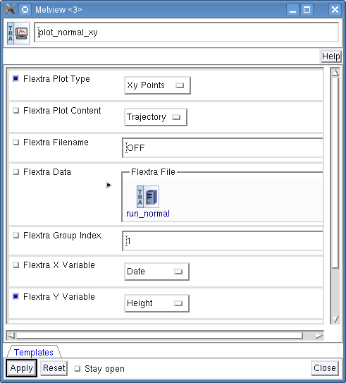
In this exercise we will display the temporal evolution of the height of the trajectories we computed in Part 3 . We will generate a graph plot with having the date as the horizontal axis and the height as the vertical axis. We will work in folder 'normal' again.
Creating a FLEXTRA Visualiser Icon
The visualisation is based on the FLEXTRA Visualiser icon just like in the case of the map-based plotting in the previous exercise (Part 4 ).
...
After these modifications your icon editor should look like this.
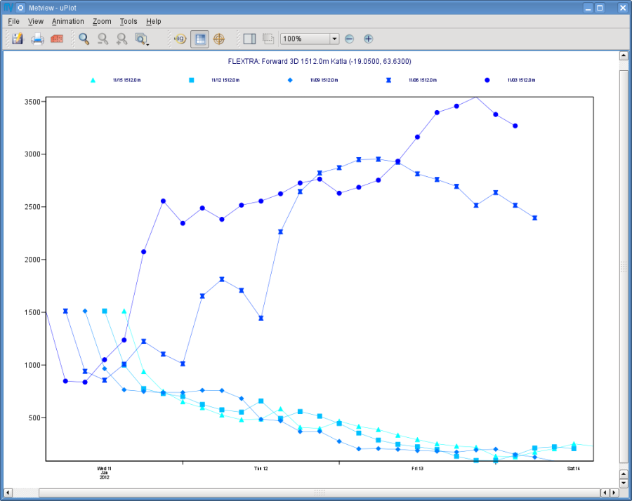
Visualising the Icon
Save your FLEXTRA Visualiser icon (Apply) then right-click and visualise to plot the trajectories.

The Metview Display Window is popping up using a custom visualisation assigned to FLEXTRA files. The title and a legend have been built exactly in the same way as in the map-based visualisation (see Part 4 ).
Customising the Plot
Our plot was generated by using hard-coded symbol plotting settings for trajectory rendering. We can change these settings exactly in the same way as we did for our map-based plot (see Part 4 for details). Now we will not create a new icon but simply reuse the Symbol Plotting icon called 'symbol' we created in Part 4 . Drop this icon into the plot to see the effect of the settings.
Changing the View
We will further customise the plot by changing the axis value ranges and adding axis labels and grid-lines to it. To change these properties we need a Cartesian View icon. This time you do not need to create a new icon since there is one called 'xy_view' already prepared for you. Edit his icon to see how the view is constructed (please note that the axis properties are defined via the embedded Horizontal Axis and Vertical Axis icons). Then simply drag it into the Display Window and see how you plot has been changed.
...
In this exercise we will see how to compute backward trajectories with FLEXTRA in NORMAL run mode. We will work in folder 'normal' again.
Creating a FLEXTRA Run Icon
Copy your 'run_normal' FLEXTRA Run icon (either right-click + duplicate, or drag with the middle mouse button), and rename the duplicate 'run_normal_back' by clicking on its title. Open its editor and start editing the date and time related parameters (the input data parameters are already set correctly for us so we do not need to change them):
...
We selected Reading as the end point and set the height to 1500 metres. We defined the trajectory type to be three-dimensional.
Running FLEXTRA
Save your FLEXTRA Run icon (Apply) then right-click and execute to start the trajectory computations. Within a minute (it might take longer on your machines) the icon should turn green indicating that the run was successful and the results have been cached. Right-click and examine the icon to look at its content. Please note that the first data column contains negative values indicating that we computed backward trajectories.

Visualising the Results
We can visualise the results in exactly the same way as we did in the previous chapter.
...
In this exercise we will see how to compute trajectories with FLEXTRA in CET run mode. In this mode we can generate a set of trajectories starting from the points of a uniform three-dimensional grid. Please open folder 'cet' inside 'flextra_tutorial' to start the work.
Creating a FLEXTRA Run Icon
Create a new FLEXTRA Run icon and rename it 'run_cet' then open its editor.
...
With these settings we defined a horizontal grid with only one point (exactly at the position of volcano Katla) and specified four vertical layers from 1500 to 3000 m above seal level.
Running FLEXTRA
Save your FLEXTRA Run icon (Apply) then right-click and execute to start the trajectory computations. Within a minute (it might take longer on your machines) the icon should turn green indicating that the run was successful and the results have been cached. Right-click and examine the icon to look at its content.
Visualising the Results
We can visualise the results in exactly the same way as we did in the previous chapters.
...
In this exercise we will see how to compute trajectories with FLEXTRA in FLIGHT run mode. In this mode, we can specify the starting location and starting time for each trajectory individually. It is useful to calculate, for instance, trajectories along the flight track of an aircraft. Please open folder 'flight' inside 'flextra_tutorial' to start the work.
Creating a FLEXTRA Run Icon
Create a new FLEXTRA Run icon and rename it 'run_flight' then open its editor.
First, we need to set the input data parameters (in the same way as we did it in Part 3 ):
...
Here we set the trajectory mode to 'FLIGHT' and defined an imaginary flight track called 'track' with 3 points each being valid at a different time.
Running FLEXTRA
Save your FLEXTRA Run icon (Apply) then right-click and execute to start the trajectory computations. Within a minute (it might take longer on your machine) the icon should turn green indicating that the run was successful and the results have been cached. Right-click and examine the icon to look at its content.
Visualising the Results
We can visualise the results in exactly the same way as we did in the previous chapter.
...
In this example we will write the macro equivalent of the exercise we solved in Part 3 and Part 4 : we will compute forward trajectories with FLEXTRA in the NORMAL run mode and then visualise them. Please open folder 'normal' inside 'flextra_tutorial' to start the work.
Basics
The implementation of FLEXTRA-related operations in Metview macro follow the same principles as in the interactive mode. In macro we work with the macro command equivalents of the FLEXTRA icons we have seen so far:
...
There is also a macro equivalent command for icon FLEXTRA Prepare, which is used to prepare input data for FLEXTRA. Please see Appendix A for details on it.
Automatic macro generation
The quickest way to generate a macro is to simply save a visualisation on screen as a Macro icon. Visualise your 'plot_normal' FLEXTRA Visualiser icon again and click on the macro icon in the tool bar of the Display Window.

Now a new Macro icon called 'MacroFrameworkN' is generated in your folder. Right-click visualise this icon. Now you should see your original plot reproduced.
Please note that this macro is to be used primarily as a framework. Depending on the complexity of the plot macros generated in this way may not work as expected and in such cases you may need to fine-tune them manually. So, we will use an alternative way and write our macro in the macro editor.
Step 1 - Writing a macro
Since we already have all the icons for our example we will not write the macro from scratch but instead we drop the icons into the Macro editor and just re-edit the automatically generated code.
...
Now, if you execute this macro (right-click execute or click on the Play button in the Macro editor), Metview will run FLEXTRA to compute the trajectories and you should see a Display Window popping up with the default FLEXTRA visualisation.
Step 2 - Saving and Reading FLEXTRA Data
Duplicate the 'step1' Macro icon (right-click duplicate) and rename the duplicate 'step2'. In this step we will see how to save (write) our FLEXTRA results into a file and read it back into a local variable in order to avoid restarting the FLEXTRA computations every time we change something in the macro.
...
Run this macro to make sure that it is working (a FLEXTRA File icon called 'res_normal_macro.txt' should appear in the folder). Then run it again to see that the execution time really became shorter because we bypassed the FLEXTRA trajectory computations.
Step 3 - Customising the Visualisation
Duplicate the 'step2' Macro icon (right-click duplicate) and rename the duplicate 'step3'. In this step we will change our symbol plotting settings and the map area as well.
...
In this example we will see how to read metadata and data from our FLEXTRA outputs. We will get to know the usage of two FLEXTRA-specific macro functions: flextra_group_get() and flextra_tr_get(), respectively. Please open folder 'metadata' in folder 'flextra_tutorial' to start the work.
Step 1 - Using Group Metadata
In this exercise we will read some metadata from our FLEXTRA output and use it to customise our plot's title.
...