from Magics.macro import *
#setting the output
output = output(
output_formats = ['png'],
output_name = "traj_step5",
output_name_first_page_number = "off"
)
#settings of the geographical area
area = mmap(subpage_map_projection="cylindrical",
subpage_lower_left_longitude=-110.,
subpage_lower_left_latitude=20.,
subpage_upper_right_longitude=-30.,
subpage_upper_right_latitude=70.,
)
#settings of the caostlines
coast = mcoast(map_coastline_land_shade = "on",
map_coastline_land_shade_colour = "cream",
map_grid_line_style = "dash",
map_grid_colour = "grey",
map_label = "on",
map_coastline_colour = "grey")
#Load the data
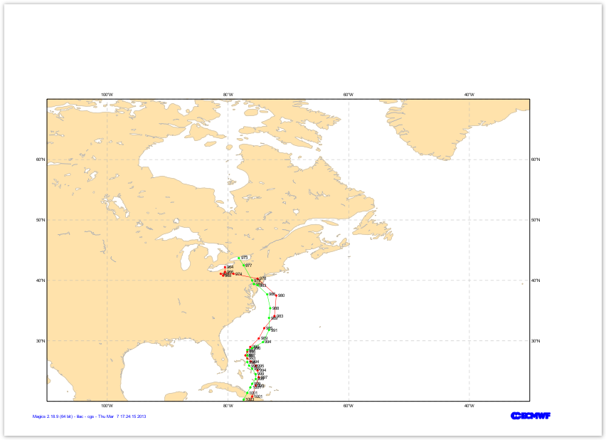
data1 = mtable(table_filename = "trajectory_01.csv",
table_variable_identifier_type='index',
table_latitude_variable = "1",
table_longitude_variable = "2",
table_value_variable = "6",
table_header_row = 0,
)
#Define the symbol plotting with connected
line1=msymb(symbol_type='markerboth',
symbol_marker_index = 28,
symbol_colour = "red",
symbol_height = 0.20,
symbol_text_font_colour = "black",
symbol_connect_line ='on'
)
#Load the data
data2 = mtable(table_filename = "trajectory_02.csv",
table_variable_identifier_type='index',
table_latitude_variable = "1",
table_longitude_variable = "2",
table_value_variable = "6",
table_header_row = 0,
)
#Define the symbol plotting with connected
line2=msymb(symbol_type='both',
symbol_marker_index = 28,
symbol_colour = "green",
symbol_height = 0.20,
symbol_text_font_colour = "black",
symbol_connect_line ='on'
)
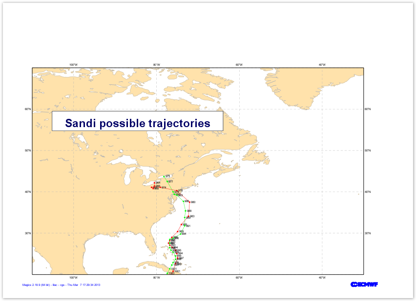
text = mtext(
text_lines= ["<font colour='navy'> Sandi possible trajectories </font>"],
text_justification= 'centre',
text_font_size= 1.,
text_font_style= 'bold',
text_box_blanking='on',
text_border='on',
text_mode='positional',
text_box_x_position = 3.,
text_box_y_position = 12.,
text_box_x_length = 13.,
text_box_y_length = 1.5,
text_border_colour='charcoal')
plot(output, area, coast, data1, line1, date2data2, line2, text) |