Objectives
- Set-up a cylindrical projection over the United States.
- Apply land-shading on the coastlines.
- Load a CSV file containing a possible trajectory of the storm
- Apply a symbol plotting to visualise this trajectory
- Repeat for all the trajectories.
- Add a positional text
You will need to download
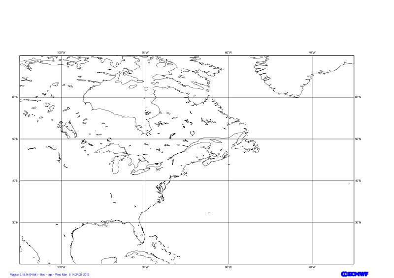
Setting of the geographical area
The Geographical area we want to work with today is defined by its lower-left corner [20oN, 110oW] and its upper-right corner [70oN, 30oW].
Have a look at the subpage documentation to learn how to set-up a projection .
from Magics.macro import *
#setting the output
output = output(
                output_formats = ['png'],
                output_name = "traj_step1",
                output_name_first_page_number = "off"
        )
#settings of the geographical area
area = mmap(subpage_map_projection="cylindrical",
        subpage_lower_left_longitude=-110.,
        subpage_lower_left_latitude=20.,
        subpage_upper_right_longitude=-30.,
        subpage_upper_right_latitude=70.,
    )
#Using a default coastlines to see the result
plot(output, area, mcoast())
Setting the coastlines
Until now you have used the mcoast to add coastlines to your plot. The mcoast object comes with a lot of parameters to allow you to style your coastlines layer.
The full list of parameters can be found in the Coastlines documentation.
In this first exercise, we will like to see:
- The land coloured in cream.
- The coastlines in grey.
- The grid as a grey dash line.
from Magics.macro import *
#setting the output
output = output(
                output_formats = ['png'],
                output_name = "traj_step2",
                output_name_first_page_number = "off"
        )
#settings of the geographical area
area = mmap(subpage_map_projection="cylindrical",
        subpage_lower_left_longitude=-110.,
        subpage_lower_left_latitude=20.,
        subpage_upper_right_longitude=-30.,
        subpage_upper_right_latitude=70.,
    )
 #settings of the caostlines
coast = mcoast(map_coastline_land_shade = "on",
      map_coastline_land_shade_colour = "cream",
      map_grid_line_style = "dash",
      map_grid_colour = "grey",
      map_label = "on",
      map_coastline_colour = "grey")
plot(output, area, coast)
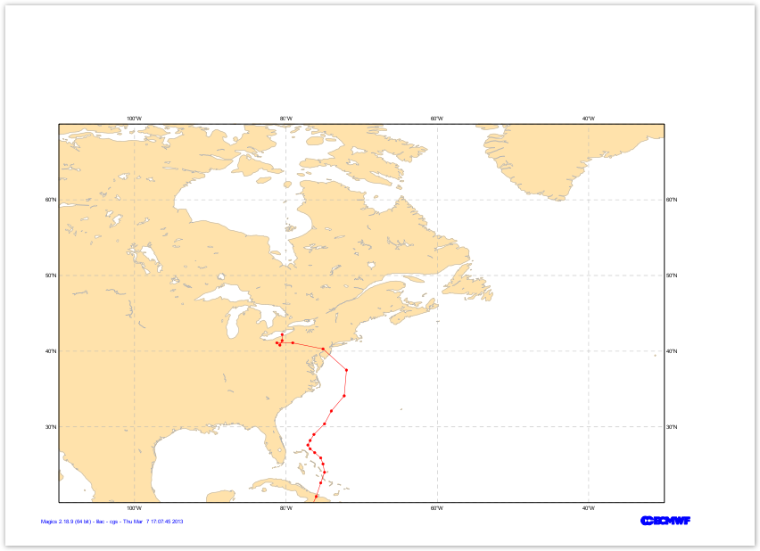
Add a first trajectory
One you have downloaded trajectories.tar, you will have 52 csv (Comma Separated Value) files, one for each possible trajectories.
13.3,-79.4,20121023,0,26,1001
13.3,-78.5,20121023,600,29,999
14.1,-78.5,20121023,1200,31,997
14.7,-78.2,20121023,1800,35,994
The first column is the latitude, the second the longitude, and the value of the pressure in in the 6th column.
This information needs to be given to Magics . This can be done with the mtable data action described in the CSV Input Documentation.
A simple Symbol Plotting using connected line will then give a nice visualisation. The full list of parameters of the msymb object can be found in the Symbol Plotting Documentation.
from Magics.macro import *
#setting the output
output = output(
                output_formats = ['png'],
                output_name = "traj_step3",
                output_name_first_page_number = "off"
        )
#settings of the geographical area
area = mmap(subpage_map_projection="cylindrical",
        subpage_lower_left_longitude=-110.,
        subpage_lower_left_latitude=20.,
        subpage_upper_right_longitude=-30.,
        subpage_upper_right_latitude=70.,
    )
 #settings of the caostlines
coast = mcoast(map_coastline_land_shade = "on",
      map_coastline_land_shade_colour = "cream",
      map_grid_line_style = "dash",
      map_grid_colour = "grey",
      map_label = "on",
      map_coastline_colour = "grey")
#Load the data
data1 = mtable(table_filename = "trajectory_01.csv",
                table_variable_identifier_type='index',
                table_latitude_variable = "1",
                table_longitude_variable = "2",
                table_value_variable = "6",
                table_header_row = 0,
                 )
#Define the symbol plotting with connected
line1=msymb(symbol_type='marker',
                symbol_marker_index = 28,
                symbol_colour = "red",
                symbol_height = 0.20,
                symbol_text_font_colour = "black",
                symbol_connect_line ='on'
                )
plot(output, area, coast, data1, line1)
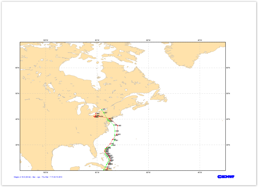
Add a second trajectory
Here, we just have to repeat the same steps, loading the file trajectory_02.csv, just changing the colour...
Try symbol_type="both..
Once done, you can repeat that for the 52 trajectories as we did in the full solution.
from Magics.macro import *
#setting the output
output = output(
                output_formats = ['png'],
                output_name = "traj_step3",
                output_name_first_page_number = "off"
        )
#settings of the geographical area
area = mmap(subpage_map_projection="cylindrical",
        subpage_lower_left_longitude=-110.,
        subpage_lower_left_latitude=20.,
        subpage_upper_right_longitude=-30.,
        subpage_upper_right_latitude=70.,
    )
 #settings of the caostlines
coast = mcoast(map_coastline_land_shade = "on",
      map_coastline_land_shade_colour = "cream",
      map_grid_line_style = "dash",
      map_grid_colour = "grey",
      map_label = "on",
      map_coastline_colour = "grey")
#Load the data
data1 = mtable(table_filename = "trajectory_01.csv",
                table_variable_identifier_type='index',
                table_latitude_variable = "1",
                table_longitude_variable = "2",
                table_value_variable = "6",
                table_header_row = 0,
                 )
#Define the symbol plotting with connected
line1=msymb(symbol_type='both',
                symbol_marker_index = 28,
                symbol_colour = "red",
                symbol_height = 0.20,
                symbol_text_font_colour = "black",
                symbol_connect_line ='on'
                )
#Load the data
data2 = mtable(table_filename = "trajectory_02.csv",
                table_variable_identifier_type='index',
                table_latitude_variable = "1",
                table_longitude_variable = "2",
                table_value_variable = "6",
                table_header_row = 0,
                 )
#Define the symbol plotting with connected
line2=msymb(symbol_type='both',
                symbol_marker_index = 28,
                symbol_colour = "green",
                symbol_height = 0.20,
                symbol_text_font_colour = "black",
                symbol_connect_line ='on'
                )
plot(output, area, coast, data1, line1, data2, line2)
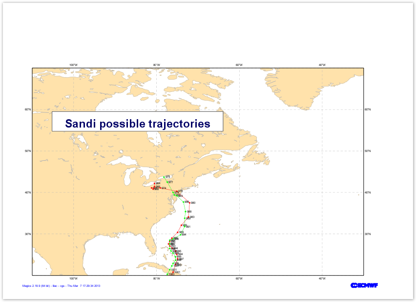
Position the text
To finish, we just want to demonstrate the possibility of adding a text box wherever you want on your page.
Remember that you can use a basic html formatting for your text. You can check the text documentation.
from Magics.macro import *
#setting the output
output = output(
                output_formats = ['png'],
                output_name = "traj_step5",
                output_name_first_page_number = "off"
        )
#settings of the geographical area
area = mmap(subpage_map_projection="cylindrical",
        subpage_lower_left_longitude=-110.,
        subpage_lower_left_latitude=20.,
        subpage_upper_right_longitude=-30.,
        subpage_upper_right_latitude=70.,
    )
 #settings of the caostlines
coast = mcoast(map_coastline_land_shade = "on",
      map_coastline_land_shade_colour = "cream",
      map_grid_line_style = "dash",
      map_grid_colour = "grey",
      map_label = "on",
      map_coastline_colour = "grey")
#Load the data
data1 = mtable(table_filename = "trajectory_01.csv",
                table_variable_identifier_type='index',
                table_latitude_variable = "1",
                table_longitude_variable = "2",
                table_value_variable = "6",
                table_header_row = 0,
                 )
#Define the symbol plotting with connected
line1=msymb(symbol_type='both',
                symbol_marker_index = 28,
                symbol_colour = "red",
                symbol_height = 0.20,
                symbol_text_font_colour = "black",
                symbol_connect_line ='on'
                )
#Load the data
data2 = mtable(table_filename = "trajectory_02.csv",
                table_variable_identifier_type='index',
                table_latitude_variable = "1",
                table_longitude_variable = "2",
                table_value_variable = "6",
                table_header_row = 0,
                 )
#Define the symbol plotting with connected
line2=msymb(symbol_type='both',
                symbol_marker_index = 28,
                symbol_colour = "green",
                symbol_height = 0.20,
                symbol_text_font_colour = "black",
                symbol_connect_line ='on'
                )
text = mtext(
        text_lines= ["<font colour='navy'> Sandi possible trajectories </font>"],
        text_justification= 'centre',
        text_font_size= 1.,
        text_font_style= 'bold',
        text_box_blanking='on',
        text_border='on',
        text_mode='positional',
        text_box_x_position = 3.,
        text_box_y_position = 12.,
        text_box_x_length = 13.,
        text_box_y_length = 1.5,
        text_border_colour='charcoal')
plot(output, area, coast, data1, line1, data2, line2, text)
Go to the next step...
Go to to the Main Magics Tutorial page...