...
The Geographical area we want to work with today is defined by its lower-left corner [20oN, 110oEW] and its upper-right corner [70oN, 30oEW].
Have a look at the subpage documentation to learn how to setup set-up a projection .
| Section |
|---|
| Column |
|---|
| | Info |
|---|
|
| Useful subpage parameters |
|---|
subpage_lower_left_longitude | | subpage_lower_left_latitude | | subpage_upper_right_longitude | | subpage_upper_right_latitude |
|
| Code Block |
|---|
| theme | Confluence |
|---|
| language | python |
|---|
| title | Python - Setting a projection |
|---|
| collapse | true |
|---|
| from Magics.macro import *
#setting the output
output = output(
output_formats = ['png'],
output_name = "maptraj_step1",
output_name_first_page_number = "off"
)
#settings of the geographical area
area = mmap(subpage_map_projection="cylindrical",
subpage_lower_left_longitude=-110.,
subpage_lower_left_latitude=20.,
subpage_upper_right_longitude=-30.,
subpage_upper_right_latitude=70.,
)
#Using a default coastlines to see the result
plot(output, area, mcoast()) |
|
| Column |
|---|
| 
|
|
...
- The land coloured in cream.
- The coastlines in grey.
- The grid as a grey dash line.
...
| Section |
|---|
| Column |
|---|
| | Info |
|---|
|
| Useful Coastlines parameters |
|---|
map_coastline_land_shade | | map_coastline_land_shade_colour | | map_coastline_colour | | map_grid_colour | | map_grid_line_style |
|
| Code Block |
|---|
| theme | Confluence |
|---|
| language | python |
|---|
| title | Python - Coastlines |
|---|
| collapse | true |
|---|
| from Magics.macro import *
#setting the output
output = output(
output_formats = ['png'],
output_name = " |
maptraj_step2",
output_name_first_page_number = "off"
)
#settings of the geographical area
area = mmap(subpage_map_projection="cylindrical",
subpage_lower_left_longitude=-110.,
subpage_lower_left_latitude=20.,
subpage_upper_right_longitude=-30.,
subpage_upper_right_latitude=70.,
)
#settings of the caostlines
coast = mcoast(map_coastline_land_shade = "on",
map_coastline_land_shade_colour = "cream",
map_grid_line_style = "dash",
map_grid_colour = "grey",
map_label = "on",
map_coastline_colour = "grey")
plot(output, area, coast) |
|
| Column |
|---|
| Image Modified |
|
Add a first trajectory
One you have downloaded trajectories.tar, you will have 52 csv (Comma Separated Value) files, one for each possible trajectories.
| Code Block |
|---|
| title | first few lines of trajectory_01.csv |
|---|
|
13.3,-79.4,20121023,0,26,1001
13.3,-78.5,20121023,600,29,999
14.1,-78.5,20121023,1200,31,997
14.7,-78.2,20121023,1800,35,994 |
The first column is the latitude, the second the longitude, and the value of the pressure in in the 6th column.
This information needs to be given to Magics . This can be done with the mtable data action described in the CSV Input Documentation.
A simple Symbol Plotting using connected line will then give a nice visualisation. The full list of parameters of the msymb object can be found in the Symbol Plotting Documentation.
| Section |
|---|
| Column |
|---|
| | Info |
|---|
|
| Useful input parameters |
|---|
table_filename | | table_variable_identifier_type | | table_latitude_variable | | table_longitude_variable | | table_value_variable |
| Useful Symbol parameters |
|---|
symbol_type | | symbol_marker_index | | symbol_connect_line |
|
| Code Block |
|---|
| theme | Confluence |
|---|
| language | python |
|---|
| title | Python - CSV file and Symbol plotting |
|---|
| collapse | true |
|---|
| from Magics.macro import *
#setting the output
output = output(
output_formats = ['png'],
output_name = "traj_step3",
output_name_first_page_number = "off"
)
#settings of the geographical area
area = mmap(subpage_map_projection="cylindrical",
subpage_lower_left_longitude=-110.,
subpage_lower_left_latitude=20.,
subpage_upper_right_longitude=-30.,
subpage_upper_right_latitude=70.,
)
#settings of the caostlines
coast = mcoast(map_coastline_land_shade = "on",
map_coastline_land_shade_colour = "cream",
map_grid_line_style = "dash",
map_grid_colour = "grey",
map_label = "on",
map_coastline_colour = "grey")
#Load the data
data1 = mtable(table_filename = "trajectory_01.csv",
table_variable_identifier_type='index',
table_latitude_variable = "1",
table_longitude_variable = "2",
table_value_variable = "6",
table_header_row = 0,
)
#Define the symbol plotting with connected
line1=msymb(symbol_type='marker',
symbol_marker_index = 28,
symbol_colour = "red",
symbol_height = 0.20,
symbol_text_font_colour = "black",
symbol_connect_line ='on'
)
plot(output, area, coast, data1, line1) |
|
| Column |
|---|
| 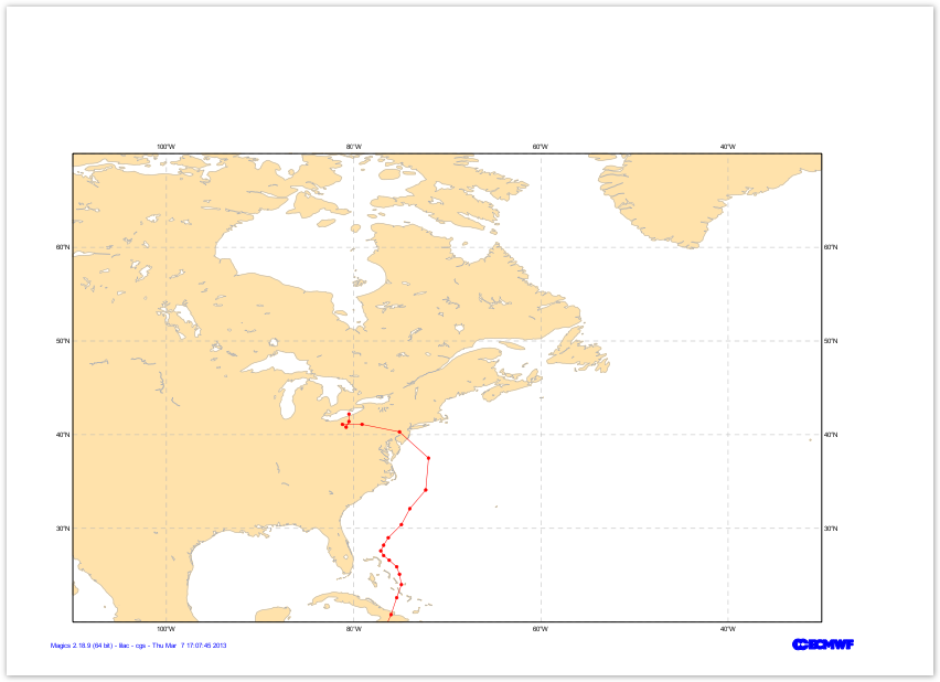 Image Added Image Added |
|
Add a second trajectory
Here, we just have to repeat the same steps, loading the file trajectory_02.csv, just changing the colour...
Try symbol_type="both..
Once done, you can repeat that for the 52 trajectories as we did in the full solution.
| Section |
|---|
| Column |
|---|
| | Info |
|---|
|
| Useful input parameters |
|---|
table_filename | | table_variable_identifier_type | | table_latitude_variable | | table_longitude_variable | | table_value_variable |
| Useful Symbol parameters |
|---|
symbol_type | | symbol_marker_index | | symbol_connect_line |
|
| Code Block |
|---|
| theme | Confluence |
|---|
| language | python |
|---|
| title | Python - CSV file and Symbol plotting |
|---|
| collapse | true |
|---|
| from Magics.macro import *
#setting the output
output = output(
output_formats = ['png'],
output_name = "traj_step3",
output_name_first_page_number = "off"
)
#settings of the geographical area
area = mmap(subpage_map_projection="cylindrical",
subpage_lower_left_longitude=-110.,
subpage_lower_left_latitude=20.,
subpage_upper_right_longitude=-30.,
subpage_upper_right_latitude=70.,
)
#settings of the caostlines
coast = mcoast(map_coastline_land_shade = "on",
map_coastline_land_shade_colour = "cream",
map_grid_line_style = "dash",
map_grid_colour = "grey",
map_label = "on",
map_coastline_colour = "grey")
#Load the data
data1 = mtable(table_filename = "trajectory_01.csv",
table_variable_identifier_type='index',
table_latitude_variable = "1",
table_longitude_variable = "2",
table_value_variable = "6",
table_header_row = 0,
)
#Define the symbol plotting with connected
line1=msymb(symbol_type='both',
symbol_marker_index = 28,
symbol_colour = "red",
symbol_height = 0.20,
symbol_text_font_colour = "black",
symbol_connect_line ='on'
)
#Load the data
data2 = mtable(table_filename = "trajectory_02.csv",
table_variable_identifier_type='index',
table_latitude_variable = "1",
table_longitude_variable = "2",
table_value_variable = "6",
table_header_row = 0,
)
#Define the symbol plotting with connected
line2=msymb(symbol_type='both',
symbol_marker_index = 28,
symbol_colour = "green",
symbol_height = 0.20,
symbol_text_font_colour = "black",
symbol_connect_line ='on'
)
plot(output, area, coast, data1, line1, data2, line2) |
|
| Column |
|---|
| 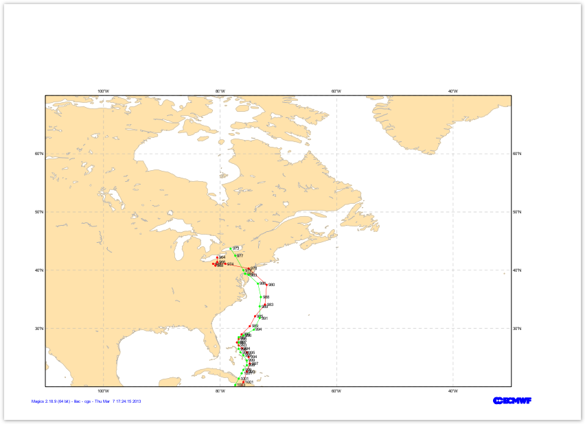 Image Added Image Added |
|
Position the text
To finish, we just want to demonstrate the possibility of adding a text box wherever you want on your page.
Remember that you can use a basic html formatting for your text. You can check the text documentation.
| Section |
|---|
| Column |
|---|
| | Info |
|---|
|
| Useful text parameters |
|---|
text_lines | | text_justification | | text_mode | | text_box_x_position | | text_box_y_position | | text_box_x_length | | text_box_x_length | | text_border | | text_box_blanking |
|
| Code Block |
|---|
| theme | Confluence |
|---|
| language | python |
|---|
| title | Python - Positionning a text |
|---|
| collapse | true |
|---|
| from Magics.macro import *
#setting the output
output = output(
output_formats = ['png'],
output_name = "traj_step5",
output_name_first_page_number = "off"
)
#settings of the geographical area
area = mmap(subpage_map_projection="cylindrical",
subpage_lower_left_longitude=-110.,
subpage_lower_left_latitude=20.,
subpage_upper_right_longitude=-30.,
subpage_upper_right_latitude=70.,
)
#settings of the caostlines
coast = mcoast(map_coastline_land_shade = "on",
map_coastline_land_shade_colour = "cream",
map_grid_line_style = "dash",
map_grid_colour = "grey",
map_label = "on",
map_coastline_colour = "grey")
#Load the data
data1 = mtable(table_filename = "trajectory_01.csv",
table_variable_identifier_type='index',
table_latitude_variable = "1",
table_longitude_variable = "2",
table_value_variable = "6",
table_header_row = 0,
)
#Define the symbol plotting with connected
line1=msymb(symbol_type='both',
symbol_marker_index = 28,
symbol_colour = "red",
symbol_height = 0.20,
symbol_text_font_colour = "black",
symbol_connect_line ='on'
)
#Load the data
data2 = mtable(table_filename = "trajectory_02.csv",
table_variable_identifier_type='index',
table_latitude_variable = "1",
table_longitude_variable = "2",
table_value_variable = "6",
table_header_row = 0,
)
#Define the symbol plotting with connected
line2=msymb(symbol_type='both',
symbol_marker_index = 28,
symbol_colour = "green",
symbol_height = 0.20,
symbol_text_font_colour = "black",
symbol_connect_line ='on'
)
text = mtext(
text_lines= ["<font colour='navy'> Sandi possible trajectories </font>"],
text_justification= 'centre',
text_font_size= 1.,
text_font_style= 'bold',
text_box_blanking='on',
text_border='on',
text_mode='positional',
text_box_x_position = 3.,
text_box_y_position = 12.,
text_box_x_length = 13.,
text_box_y_length = 1.5,
text_border_colour='charcoal')
plot(output, area, coast, data1, line1, data2, line2, text) |
|
| Column |
|---|
| 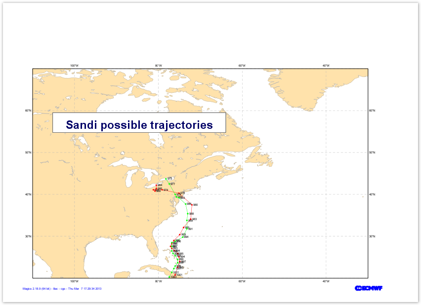 Image Added Image Added |
|
Go to the next step...
Go to to the Main Magics Tutorial page...