...
The production of seasonal forecasts, also known as seasonal climate forecasts, has undergone a huge transformation in the last few decades: from a purely academic and research exercise in the early '90s to the current situation where several meteorological forecast services, throughout the world, conduct routine operational seasonal forecasting activities. Such activities are devoted to providing estimates of statistics of weather on the monthly and seasonal and monthly time scales, which places them somewhere between conventional weather forecasts and climate predictions.
...
Each model simulates the Earth system processes that influence weather patterns in slightly different ways, makes slightly different approximations, leading to different kinds of model error. The These errors typically increase with the increase of integration time, so that the accumulated model errors become significant in comparison to the signal that the model is meant to predict. Some such errors are shared by the different models but others are not, so combining the output from a number of models enables a more realistic representation of the uncertainties due to model error. In most cases, such combined forecasts are, on average, more skilful than forecasts from the best of the individual models.
...
Seasonal forecasts are not weather forecasts: the role of the hindcasts
Due to its long leadtimes, a few months since the start date of the forecast, some systematic errors appear that can completely kill the signals that are expected to be predicted. To avoid that, seasonal forecasting systems work with a reference climate to determine how predicted values differ from what is normal for a given region and time of yearSeasonal forecasts are started from an observed state of (all components of) the climate system, which is then evolved in time over a period of a few months. Errors present at the start of the forecast (due to the imprecise measurement of the initial conditions and the approximations assumed in the formulation of the models) persist or, more often, grow through the model integration, reaching magnitudes comparable to that of the predictable signals. Some such errors are random; the effect of these on the outcome is quantified through the use of ensembles. Some errors, however, are systematic; if these systematic errors were determined, corrections could be applied to the forecasts to extract the useful information. This is achieved by comparing retrospective forecasts (hindcasts) with observations. The same forecast system is run for past dates, so that kind of model climate can be estimated, and the forecasts be bias-corrected with respect to that model climate. Those forecast runs for earlier years are known as 'hindcasts' or 're-forecasts' and they are a key concept in seasonal forecasting, in such a way that a forecast itself it's not useful without relating it with the relevant hindcasts.several starting points in the past in the same way as a forecast would be run (with only knowledge of the starting point), for the same length of time as an equivalent forecast. The resulting data set constitutes a 'climate' of the model, which can then be compared with the observed climate of the real world. The systematic differences between the model and the real world - usually referred to as biases - are thus quantified and used as the basis for corrections which can be applied to future, real-time forecasts. Given the relative magnitude of such biases, some basic corrections are essential to convert the data into forecast information - therefore a forecast by itself is not useful without relating it to the relevant hindcasts.
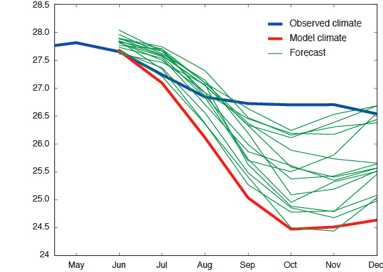
The image below is In the image shown below as an example of the crucial role of the hindcasts in seasonal forecasting, a . It shows the predicted time evolution of monthly-average of temperature in a given region is plotted. All the forecast ensemble members (green lines) seem to point to colder than usual conditions when directly compared to the observed climate (blue line). If the model climate derived from the hindcasts (red line) is taken into account the conclusion is quite different, with all the forecast ensemble members now consistently pointing to warmer than usual conditions.. The blue line represents the average conditions observed over a period in the past (the reference period; in this case, 1993-2014), for each month between May and December; the red line is the equivalent model climate average over the same reference period. The difference between the two clearly indicates a significant cold bias, increasing with the time into the forecast. An ensemble of forecasts for a particular year is shown as green lines. When compared to the observed 'normal', all green ensemble predictions are for colder-than-normal conditions - not necessarily surprising when remembering that the model is systematically colder than the real world. However, when comparison is made with the model's 'normal' (the red line), all forecast ensemble members indicate warmer-than-normal conditions. Clearly, as the forecast is an output of the model, the latter comparison is the more appropriate.
Additionally to their unavoidable role to correct those in correcting systematic errors, hindcasts are also used to assess the skill of the different seasonal forecasting systems. In that way, the real-time forecasts are expected to behave with the same skill that the system has shown for past dates, i.e. the skill shown by the hindcasts.
...