Seasonal forecasts and the Copernicus Climate Change Service (C3S)

Introduction to seasonal forecasting

The production of seasonal forecasts, also known as seasonal climate forecasts, have experienced a huge transformation in the last few decades: from a purely academic and research exercise in the early 90s to the current situation where several meteorological forecast services throughout the world conduct routine operational seasonal forecasting activities. Such activities are devoted to provide estimates of statistics of weather in the seasonal and monthly time scales, and they lie in a place somewhere between conventional weather forecasts and climate predictions.

In that sense, even though seasonal forecasts share some method and tools with weather forecasting they are part of a different paradigm which requires treating them in different ways. Seasonal forecasts instead of trying to answer to the question "how is the weather going to look like on a particular location in an specific day?", they will tell us how likely is that the coming season will be wetter, drier, warmer or colder than the usual conditions for that time of year. This kind of long term predictions are feasible due to the behaviour of some of the earth system components which evolve more slowly than the atmosphere (e.g. the ocean, the cryosphere) and in a predictable fashion, so their influence in the earth system can add a noticeable signal.

We consider here as seasonal forecasts data both the higher-frequency (sub-daily and daily) data outputs from numerical earth system weather or climate models and the derived monthly and seasonal products, up to a few months ahead of their initialization date.

Seasonal forecasting within the C3S

The C3S seasonal forecasting products are based on data from several state-of-the-art seasonal prediction systems. Multi-system combinations, as well as predictions from the individual component systems, are available. The centres currently providing forecasts to C3S are ECMWF, The Met Office and Météo-France; in the coming months data produced by Deutscher Wetterdienst and Centro Euro-Mediterraneo sui Cambiamenti Climatici will be included in the C3S multi-system.

Each model simulates the Earth system processes that influence weather patterns in slightly different ways, leading to different kinds of model error. The accumulated model errors become significant in comparison to the signal that is meant to be predicted. Some of those errors are shared by the different models but others are not, so combining the output from a number of models enables a more realistic representation of the uncertainties due to model error. The current scientific knowledge have shown that, in most cases, such combined forecasts are more skilful than forecasts from the best of the individual models.

Currently, there are graphical products available in the C3S web site and public access to the data is provided via the ECMWF WebAPI. From 2018 onwards, C3S seasonal forecast data products will be made available via the C3S Climate Data Store (CDS).

Seasonal forecasts are not weather forecasts: the role of the hindcasts

Due to its long leadtimes, a few months since the start date of the forecast, some systematic errors appear that can completely kill the signals that are expected to be predicted. To avoid that, seasonal forecasting systems work with a reference climate to determine how predicted values differ from what is normal for a given region and time of year. The same forecast system is run for past dates, so that kind of model climate can be estimated, and the forecasts be bias-corrected with respect to that model climate. Those forecast runs for earlier years are known as 'hindcasts' or 're-forecasts' and they are a key concept in seasonal forecasting, in such a way that a forecast itself it's not useful without relating it with the relevant hindcasts.

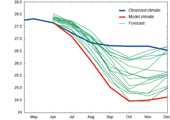
In the image shown below as an example of the crucial role of the hindcasts in seasonal forecasting, a time evolution of monthly average of temperature in a given region is plotted. All the forecast ensemble members (green lines) seem to point to colder than usual conditions when directly compared to the observed climate (blue line). If the model climate derived from the hindcasts (red line) is taken into account the conclusion is quite different, with all the forecast ensemble members now consistently pointing to warmer than usual conditions.

Additionally to their unavoidable role to correct those systematic errors, hindcasts are also used to assess the skill of the different seasonal forecasting systems. In that way, the real-time forecasts are expected to behave with the same skill that the system has shown for past dates, i.e. the skill shown by the hindcasts.

Note that for reasons related with the availability of computing resources, the hindcasts usually have fewer ensemble members per start date than the real-time forecasts, e.g. ECMWF SEAS5 5 has 51 members for the real-time forecasts, and just 25 members for the hindcasts.

Seasonal forecasting systems' versions and updates

blahblahblah (system keyword, etc)

How the seasonal forecasting systems build their ensembles? And how data are produced?

"Burst" vs. "lagged" mode

In the last few decades, in the earth system modelling it has been an established technique the use of "ensemble" runs to take into account errors due to both the uncertainty in the initial conditions and model deficiencies. This means that the forecasting systems produced a set of "slightly" different runs of the same forecast which form the members of the ensemble, in a way that the outcome of the forecasting system is not a single model output but a set of different results which allow to produce a forecast in terms of a probability distribution as opposed to a single deterministic forecast.

Different techniques are commonly used to build the different members of an ensemble forecast, but one of the most common ways to create a set of slightly different members that mainly maps the uncertainty in the initial conditions, is the use of a "lagged" approach in the start dates.

• "Burst" mode: all the members are initialized (start date) at the same value (e.g. all members initialized on 1st March 2017, this is the case for ECMWF system)
• "Lagged" mode: members are initialized in different start dates (e.g. 2 members initialized every day of the month, this is the case for Met Office system)

Among all the systems that contribute to the C3S seasonal forecasts, some of them have opted to use a "burst" mode, while some others lag the start dates of the members of their ensembles. For more details, refer to the table below in the "Production schedules" subsection

Fixed vs. on-the-fly hindcasts

Due to several reasons, from computer load balance to flexibility in the introduction of changes in the systems, the different seasonal forecast contributors to C3S use different schedules to produce their hindcast sets:

• Fixed hindcasts: Some systems are designed so their expected lifetime will be around 4-5 years. Thus, once the system has been designed and tested, its development gets frozen and exactly that version of the model is used to run all the hindcast members for the whole climate period for that model. In that way, the hindcasts are produced well in advance the real-time forecasts and they constitute a fixed dataset during the lifetime of that seasonal forecasting system
• On-the-fly hindcasts: Some other systems run the necessary set of hindcasts every time they produce a new real-time forecast. They are produce just slightly in advance (a few weeks) the real-time forecast and using exactly the same version of the forecasting system. In this way changes in the system can be introduced more frequently and the computing of the hindcasts can be spanned over a longer period, then balancing the load of the computing resources.

Production schedules in the seasonal forecasting systems contributing to C3S

Table with production per system and per forecast/hindcast type

Description of the c3s-seasonal dataset in the MARS archive

Data tree

MMSF

MSMM

MMSA

*** Note: check EUROSIP documentation (it is said that MMSA is not calculated for "lagged" ensembles)

(*) Due to some peculiarities of GRIB formatting and MetOffice forecasting system design, the value of the MARS keyword SYSTEM is changed on a yearly basis, so it has no direct relation with the model version of their system

Table 1: Values of the MARS keyword SYSTEM for the operational C3S seasonal contributors

High frequency data (stream MMSF)

TYPE=fc (hidden)

YEAR (note, hindcasts formally equivalent to forecasts)

MONTH

ORIGIN (ecmf, lfpw, egrr)

SYSTEM (hidden, usually... always [are we going to have at some point different systems for the same start date... e.g. MetOffice]?)

LEVTYPE (sfc, plev)

DATE (it is hidden for ecmf, lfpw and 1st of the current month for egrr)

Leaf contents: number, step (freq= 6h, 24h, 12h), [level], parameter

Monthly means and other monthly statistics (stream MSMM)

Derived probability products

TYPE  (em, ensemble mean; hcmean: hindcast climate mean, one for every real-time forecast)

ORIGIN

SYSTEM (optional)

LEVTYPE (sfc, plev)

Leaf contents: date, time***, fcmonth, [level], parameter

*** Ask Manuel, why time is not "hidden" in the final leaf (as it is for MMSF) 

Derived forecast products

TYPE (fcmean/max/min/stdev: "Forecast mean,...")

YEAR (note, hindcasts formally equivalent to forecasts)

ORIGIN

SYSTEM (optional)

LEVTYPE (sfc, plev)

Leaf contents: date, time***, fcmonth, number, [level], parameter

*** Ask Manuel, why time is not "hidden" in the final leaf (as it is for MMSF) 

Real-time forecasts monthly anomalies (stream MMSA)

Derived probability products

TYPE  (em, ensemble mean)

ORIGIN

SYSTEM (optional)

LEVTYPE (sfc, plev)

Leaf contents: date, time***, fcmonth, [level], parameter

*** Ask Manuel, why time is not "hidden" in the final leaf (as it is for MMSF) 

Derived forecast products

TYPE (fcmean "Forecast mean")

ORIGIN

SYSTEM (optional)

LEVTYPE (sfc, plev)

Leaf contents: date, time***, fcmonth, number, [level], parameter

*** Ask Manuel, why time is not "hidden" in the final leaf (as it is for MMSF)