CMIP6: Global climate projections

Last modified on Dec 12, 2023 09:53

Introduction

What are global climate projections?

Global climate projections are simulations of the climate system performed with general circulation models which represent physical processes in the atmosphere, ocean, cryosphere and land surface. These models cover the entire globe and use information about the external influences on the system. Such simulations have been generated by multiple independent climate research centres in an effort coordinated by the World Climate Research Program (WCRP) and assessed by the Intergovernmental Panel on Climate Change (IPCC). These climate projections underpin the conclusions of the IPCC Assessment Reports that “Continued emission of greenhouse gases will cause further warming and long-lasting changes in all components of the climate system, increasing the likelihood of severe, pervasive and irreversible impacts for people and ecosystems”.

The Climate Model Intercomparison Project (CMIP)

The Climate Model Intercomparison Project (CMIP) was established in 1995 by the World Climate Research Program (WCRP) to provide climate scientists with a database of coupled Global Circulation Model (GCM) simulations.

 The CMIP process involves institutions (such as national meteorological centres or research institutes) from around the world running their climate models with an agreed set of input parameters (forcings). The modelling centres produce a set of standardised output. When combined, these produce a multi-model dataset that is shared internationally between modelling centres and the results compared.

 Analysis of the CMIP data allows for

• an improved understanding of the climate, including its variability and change,
• an improved understanding of the societal and environmental implications of climate change in terms of impacts, adaptation and vulnerability,
• informing the Intergovernmental Panel on Climate Change (IPCC) reports.

Comparison of different climate models allows for

• determining why similarly forced models produce a range of responses,
• evaluating how realistic the different models are in simulating the recent past,
• examining climate predictability.

CMIP6

The sixth phase of the Coupled Model Intercomparison Project (CMIP6) consists of 134 models from 53 modelling centres (Durack, 2020). CMIP6 data publication began in 2019 and the majority of the data publication was completed in 2022. The scientific analyses from CMIP6 will be used extensively in the Intergovernmental Panel on Climate Change (IPCC) 6th Assessment Report (AR6), due for release in 2021/22 (IPCC, 2020).

CMIP6 aims to address 3 main questions:

• How does the Earth system respond to forcing?
• What are the origins and consequences of systematic model biases?
• How can we assess future climate changes given internal climate variability, predictability, and uncertainties in scenarios (Eyring et al, 2016)?

There are some differences between the experimental design and organisation of CMIP6 and its predecessor CMIP5. It was decided that for CMIP6, a new and more federated structure would be used, consisting of the following three major elements:

1. A handful of common experiments, the DECK (Diagnostic, Evaluation and Characterization of Klima) and CMIP historical simulations (1850 – near-present) that will maintain continuity and help document basic characteristics of models across different phases of CMIP;
2. Common standards, coordination, infrastructure and documentation that will facilitate the distribution of model outputs and the characterization of the model ensemble;
3. An ensemble of CMIP-Endorsed Model Intercomparison Projects (MIPs) that will be specific to a particular phase of CMIP (now CMIP6) and that will build on the DECK and CMIP historical simulations to address a large range of specific questions and fill the scientific gaps of the previous CMIP phases (World Climate Research Programme, 2020).

The CMIP6 data archive is distributed through the Earth System Grid Federation (ESGF) though many national centres have either a full or partial copy of the data. A quality-controlled subset of CMIP6 data are made available through the Climate Data Store (CDS) for the users of the Copernicus Climate Change Service (C3S).

Global climate projections in the CDS

The global climate projections in the Climate Data Store (CDS) are a quality-controlled subset of the wider CMIP6 data. These data represent only a small subset of CMIP6 archive. A set of 51 core variables from the CMIP6 archive were identified for the CDS. These variables are provided from 9 of the most popular CMIP6 experiments. These data can be used to assess plausible future changes in the variables provided, under a range of socio-economic pathways.

The CDS subset of CMIP6 data has been through a quality control procedure which ensures a high standard of dependability of the data. Additional data can be found in the main CMIP6 ESGF archive, however these data come with very limited quality assurance and may have metadata errors or omissions.

Experiments

Shared Socioeconomic Pathway (SSP) Experiments

The SSP scenario experiments can be understood in terms of two pathways, a Shared Socioeconomic Pathway (SSP) and a Representative Concentration Pathway (RCP). The two pathways are represented by the three digits that make up the experiment’s name. The first digit represents the SSP storyline for the socio-economic mitigation and adaptation challenges that the experiment represents (Figure 1). The second and third digits represent the RCP climate forcing that the experiment follows. For example, experiment ssp245 follows SSP2, a storyline with intermediate mitigation and adaptation challenges, and RCP4.5 which leads to a radiative forcing of 4.5 Wm^-2 by the year 2100.

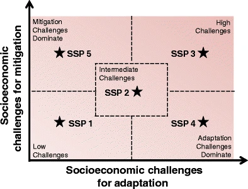
Figure 1 - The socioeconomic “Challenge Space” to be spanned by the CMIP6 SSP experiments (O’Neil et al. 2014).

Experiments in the CDS

The CDS-CMIP6 subset consists of the CMIP6 experiments detailed in the table below.

Models, grids, calendars, and pressure levels

Models 

The models included in the CDS-CMIP6 subset are detailed in the table below including a brief description of the model, further details can be found on the Earth System Documentation site (ES-DOC) or WDC-climate pages. Sometimes there are differences between the model details reported in the CMIP6 metadata and the source documentation, the models with such discrepancies are marked here with an asterix and further details are provided in a second table below. The grid IDs reported in the final column are explained further under the 'grids' section.

Grids

CMIP6 data is available either on the model’s native grid or re-gridded to one or more target grids with data variables generally provided near the centre of each grid cell (rather than at the boundaries). This re-gridding is normally done for models which use native grids other than regular lat-lon grids (e.g. cubed sphere or gaussian), in these cases the output has been re-gridded to a regular lat-lon grid by the modelling centers. For CMIP6 there is a requirement to record both the native grid of the model, and the approximate resolution of the final output data (archived in the CMIP6 repository, and available via the CDS) as a “nominal_resolution”.  This "nominal_resolution” enables users to identify which models have relatively high resolution output. Information about the grids can be found in the model table above, under 'Model Details', and within the NetCDF file metadata.

The column 'Grids on the CDS ('gn', 'gr' or 'gr1')' lists which grid IDs are associated with the data from that model available on the CDS. These labels reflect whether a given set of model data (variable) uploaded to ESGF is on the 

• native grid of the model component ('gn'),
• regridded to the regular target grid specified for the particular variable ('gr'),
• or another target grid ('gr1').

The output from some models has multiple different grid IDs associated with it, due to different model components (atmosphere, land, ocean, cryosphere etc.) being treated differently. This does not necessarily mean the data itself is on a different grid, for example the atmospheric variables maybe on a regular native grid ('gn'), and the ocean variables with an irregular native grid may have been regridded to the atmosphere grid (hence are labelled 'gr'), so they are on the same grid in spite of the fact that their grid ID is different. On the other hand, if a model is only listed as having output on the native grid ('gn'), this does not guarantee that all the data (variable) is on the same grid, as the native grid for different model components can be different.

Note: some data (i.e. variables) have been submitted to ESGF on multiple grids, in these cases only one grid is made available on the CDS (this is decided on a case-by-case basis).

Calendars

Climate models sometime use different calendars, for example Hadley Centre models in CMIP6 use a 360 day calendar, where every month has exactly 30 days. Some models use a fixed 365-day calendar, and others include leap-years. These variations can result in different length time-dimensions if daily data is downloaded, depending on the time period and models selected, or even failed data requests. Users need to be careful, when using the CDS user interface download form or API, to avoid selecting days which may not be available in the calendar of the given model (for example requests referring to day 31 for the Hadley Centre models would fail, because they have a 360 day calendar). The CDS form for CMIP6 currently assumes a standard calendar, so allows the selection of such missing days, and conversely may not allow selection of all days from models with non-standard calendars (but this data can be retrieved using the API). 

Pressure levels

For pressure level data the model output is available on the pressure levels according to the table below. Note that since the model output is standardised all models produce the data on the same pressure levels.

Ensembles

Each modelling centre typically run the same experiment using the same model with slightly different settings several times to confirm the robustness of results and inform sensitivity studies through the generation of statistical information. A model and its collection of runs is referred to as an ensemble. Within these ensembles, four different categories of sensitivity studies are done, and the resulting individual model runs are labelled by four integers indexing the experiments in each category

e.g. r<W>i<X>p<Y>f<Z>, where W, X, Y and Z are positive integers as defined below:

• The first category, labelled realization_index (referred to with letter r), performs experiments which differ only in random perturbations of the initial conditions of the experiment. Comparing different realizations allow estimation of the internal variability of the model climate.
• The second category, labelled initialization_index (referred to with letter i), refers to variation in initialisation parameters. Comparing differently initialised output provides an estimate of how sensitive the model is to initial conditions.
• The third category, labelled physics_index (referred to with letter p), refers to variations in the way in which sub-grid scale processes are represented. Comparing different simulations in this category provides an estimate of the structural uncertainty associated with choices in the model design.
• The fourth category labelled forcing_index (referred to with letter f) is used to distinguish runs of a single CMIP6 experiment, but with different forcings applied.

Parameter listings

Time-Independent parameters are marked with a dash in the time resolution column. Please note that some parameters defined at pressure levels, such as 1000 hPa temperature, may contain missing data where they are not defined (so the fields look incomplete over terrain) or are filled with interpolated values (different modelling centres may have different approaches). This happens when the pressure level falls below the orography.

Data Format

The CDS subset of CMIP6 data are provided as NetCDF files. NetCDF (Network Common Data Form) is a file format that is freely available and commonly used in the climate modelling community. See more details:  What are NetCDF files and how can I read them

 A CMIP6 NetCDF file in the CDS contains:

• Global metadata: these fields can describe many different aspects of the file such as
  • when the file was created
  • the name of the institution and model used to generate the file
  • Information on the horizontal grid and regridding procedure
  • links to peer-reviewed papers and technical documentation describing the climate model,
  • links to supporting documentation on the climate model used to generate the file,
  • software used in post-processing.
• variable dimensions: such as time, latitude, longitude and height
• variable data: the gridded data
• variable metadata: e.g. the variable units, averaging period (if relevant) and additional descriptive data

File naming conventions

When you download a CMIP6 file from the CDS it will have a naming convention that is as follows:

<variable_id>_<table_id>_<source_id>_<experiment_id>_<variant_label>_<grid_label>_<time_range>.nc

 Where:

• variable_id: variable is a short variable name, e.g. “tas” for “temperature at the surface”.
• table_id: this refers to the MIP table being used. The MIP tables are used to organise the variables. For example, Amon refers to monthly atmospheric variables and Oday contains daily ocean data.
• source_id: this refers to the model used that produced the data.
• experiment_id: refers to the set of experiments being run for CMIP6. For example, PiControl, historical and 1pctCO2 (1 percent per year increase in CO2).
• variant_label: is a label constructed from 4 indices (ensemble identifiers) r<W>i<X>p<Y>f<Z>, where W, K, Y and Z are integers.
• grid_label: this describes the model grid used. For example, global mean data (gm), data reported on a model's native grid (gn) or regridded data reported on a grid other than the native grid and other than the preferred target grid (gr1).
• time_range: the temporal range is in the form YYYYMM[DDHH]-YYYY[MMDDHH], where Y is year, M is the month, D is day and H is hour. Note that day and hour are optional (indicated by the square brackets) and are only used if needed by the frequency of the data. For example, daily data from the 1st of January 1980 to the 31st of December 2010 would be written 19800101-20101231.

Quality control of the CDS-CMIP6 subset

The CDS subset of the CMIP6 data have been through a set of quality control checks before being made available through the CDS. The objective of the quality control process is to ensure that all files in the CDS meet a minimum standard. Data files were required to pass all stages of the quality control process before being made available through the CDS. Data files that fail the quality control process are excluded from the CDS-CMIP6 subset, data providers are contacted and if they are able to release a new version of the data with the error corrected then providing this data passes all remaining QC steps may be available for inclusion in the next CMIP6 data release.

 The main aim of the quality control procedure is to check for metadata and gross data errors in the CMIP6 files and datasets. A brief description of each of the QC checks is provided here:

1. CF-Checks: The CF-checker tool checks that each NetCDF4 file in a given dataset is compliant with the Climate and Forecast (CF) conventions, compliance ensures that the files are interoperable across a range of software tools. When CF-checker 1.7 is run on the current data some remaining issues are highlighted, particularly for lat, lon and time bounds.
2. PrePARE: The PrePARE software tool is provided by PCMDI (Program for Climate Model Diagnosis and Intercomparison) to verify that CMIP6 files conform to the CMIP6 data protocol. All CMIP6 data should meet this required standard however this check is included to ensure that all data supplied to the CDS have passed this QC test.
3. nctime: The nctime checker checks the temporal axis of the NetCDF files. For each NetCDF file the temporal element of the file is compared with the time axis data within the file to ensure consistency. For a time-series of data comprised of several NetCDF files nctime ensures that the entire timeseries is complete, that there are no temporal gaps or overlaps in either the filename or in the time axes within the files.
4. Errata: The dataset was checked to ensure that no outstanding Errata record existed at the time of publication.
5. Data Ranges: A set of tests on the extreme values of the variables are performed, this is used to ensure that the values of the variables fall into physically realistic ranges.
6. Handle record consistency checks: This check ensures that the version of the dataset used is the most recently published dataset by the modelling centre, it also checks for any inconsistency in the ESGF publication and excludes any datasets that may have inconsistent high-level metadata.
7. Exists at all partner sites: It is asserted that each dataset exists at all three partner sites CEDA, DKRZ and IPSL.

It is important to note that passing these quality control tests should not be confused with validity: for example, it will be possible for a file to pass all QC steps but contain errors in the data that have not been identified by either data providers or data users.

 In cases where the quality control picks up errors that are related to minor technical details of the conventions, or behavior that is in line with expectations for climate model output despite being unexpected in a physical system, the data will be published with details of the errors referenced in the documentation. An example of the 2^nd type of error is given by negative salinity values which occur in one model as a result of rapid release of fresh water from melting sea-ice. These negative values are part of the noise associated with the numerical simulation and reflect what is happening in the numerical model.

Citation, license and PID information

In general the CMIP6 data Citation Service provides information for users on how to cite CMIP6 data and also information on the data licenses.

The users can decide on what level they want to refer to the CMIP6 datasets. 

The highest level is the one provided by the CDS with the use of the following DOI: 10.24381/cds.c866074c (available also at the right-hand-side of the entry). The users can refer to any data with this DOI, which are available in the CMIP6 catalogue entry in the CDS.

The CMIP6 citation Search is at http://bit.ly/CMIP6_Citation_Search. Citations for CDS CMIP6 data available in the CDS are discoverable in the ESGF on model and experiment levels (please note that these linked files are csv files, which can be looked at after downloading them). 

The CMIP6 datasets are also labelled by the so called Persistent Identifiers (PIDs). PIDs are assigned to each version of every file and dataset. These are unique identifiers of the data and they are available in the header of the netcdf datafiles. The PIDs are also provided on dataset and file levels (please note that these files are csv files, which can be looked at after downloading them).

Known issues

CDS users are directed to the CMIP6 ES-DOC Errata Service for known issues with the wider CMIP6 data pool. Data that is provided to the CDS either should not contain any errors, or minor errors should be listed in the Errata Service. Additionally, the Errata Service is also a useful resource for CDS users as data may have been withheld from the CDS for justifiable reasons.

Some models currently have either missing historical or scenario data for some variables, which is in the process of being resolved. Some details are given in the table below:

Subsetting and downloading data

CDS users will now be able to apply temporal and spatial subsetting operations to CMIP6 datasets. This mechanism (the "roocs" WPS framework) that runs at each of the partner sites: CEDA, DKRZ and IPSL. The WPS can receive requests for processing based on dataset identifiers, a temporal range, a bounding box and a range of vertical levels. Each request is converted to a job that is run asynchronously on the processing servers at the partner sites. NetCDF files are generated and the response contains download links to each of the files. Users of the CDS will be able to make subsetting selections using the web forms provided by the CDS catalogue web-interface. More advanced users will be able to define their own API requests in the CDS Toolbox that will call the WPS. Output files will be automatically retrieved so that users can access them directly within the CDS.

When CMIP6 data is downloaded from the Climate Data Store, information about any additional processing applied to the data (such as temporal or spatial subsetting) is included in both PNG and JSON form. These provenance files will be zipped up with the retrieved data and named provenance.png and provenance.json, which describe the software used and the methods applied to the data following the W3C PROV standard. For more information about how to interpret these files, please see https://rook-wps.readthedocs.io/en/latest/prov.html.

Additional resources

A training resource in python is available via a Jupyter Notebook on the C3S data tutorials page here: https://ecmwf-projects.github.io/copernicus-training-c3s/projections-cmip6.html

References

Durack, P J. (2020) CMIP6_CVs. v6.2.53.5. Available at: https://github.com/WCRP-CMIP/CMIP6_CVs (Accessed: 26 October 2020).

Eyring, V. et al. (2016) ‘Overview of the Coupled Model Intercomparison Project Phase 6 (CMIP6) experimental design and organization’, Geoscientific Model Development, 9(5), pp. 1937–1958. doi: 10.5194/gmd-9-1937-2016.

IPCC (2020) Sixth Assessment Report. Available at: https://www.ipcc.ch/assessment-report/ar6/ (Accessed: 26 October 2020).

Moss, R. et al. (2008) ‘Towards New Scenarios for Analysis of Emissions, Climate Change, Impacts, and Response Strategies’, Intergovernmental Panel on Climate Change, Geneva, pp. 132.

O’Neill, B.C. et al. (2014) ‘A new scenario framework for climate change research: the concept of shared socioeconomic pathways.’, Climatic Change, 122, pp. 387–400. doi: https://doi.org/10.1007/s10584-013-0905-2

World Climate Research Programme (2020) CMIP Phase 6 (CMIP6): Overview CMIP6 Experimental Design and Organization. Available at: https://www.wcrp-climate.org/wgcm-cmip/wgcm-cmip6 (Accessed: 2 November 2020).

Related articles

• Page:
  CORDEX: Regional climate projections
• Page:
  CMIP6: Global climate projections
• Page:
  CMIP6: Decadal climate predictions
• Page:
  CMIP: Global climate projections
• Page:
  C3S Climate projections