Overview
There are two steps required in an AI forecast system:
- First phase; supply a set of algorithms that relate initial data with predicted data for a certain time in the future. This is accomplished using Machine Learning (ML) and is done once only with the introduction of each new Cycle and associated reanalysis data.
- Second phase; use these algorithms to predict data for a certain time in the future using observed and analysed data. This is accomplished using Artificial Intelligence (AI) forecasting and can be done many times or as frequently as a forecast is required.
Machine Learning (ML)
The aim of Machine Learning (ML) is to develop (or train) an empirical model directly from observations or reanalyses. Observations implicitly contain the physics of the atmosphere but it is not necessary for ML models emulate the underpinning physics that dictates the evolution of variables through a forecast. During the ML training process, ML considers all the set of observed or initial data, and using statistical methods relates these to observed variable (e.g.temperature) six hours later at each point. The initial data and corresponding data at the end of the forecast period have been extracted from some 20 years of ERA5 data. At ECMWF, machine learning training is aimed towards producing six hour forecasts. Table2.2.1 gives the set of observed and forecast variables and the constants considered during the machine learning process at ECMWF.
Machine Learning Process
At each grid point the set of observed data is processed using the set of random weighting functions for each parameter. Initially the forecast value will not agree with those observed at the verifying time of the forecast. The error (loss function) as measured by some error metric is fed backwards (back propagation) within the process. In response, the influence of types of observations (say wind, 50hPa temperature, etc.) may be reduced while that of others (say surface temperature) may be increased. This process is repeated many times with the aim to progressively minimise the error metric (See Fig2.2.1-1).
The process incrementally improves the relationship between the set of initial observations and forecast values of a single variable for the later time. In this way a relatively simple relationship between initial data and forecast data for six hours in the future is gradually built up. This consists of probabilities of influence of each meteorological parameter in the form of a weighting for each input data type. Taking all the weighting functions together forms an algorithm for use during the AI forecasts.
ML when completed returns weights for all variables that give the best forecast at T+6. These weights are different according to the variable being forecast (e.g. the weight given to surface pressure used in calculating a forecast surface temperature is different from weight given to surface pressure used in calculating a forecast surface dew point). These relationships are in the form of a set of algorithms that can be used by subsequent AI forecasts.
Sometimes the ML model requires fine-tuning. This process doesn't require a full retraining of the model. Instead, targeted adjustments to the model's weights and parameters reflect the new data and scientific findings. This selective updating helps ensure that the new information is not drowned out by the volume of pre-existing training data and avoids conflicts with established reanalyses. This keeps ECMWF ML models at the cutting edge.
Artificial Intelligence (AI) forecasting
The aim of AI forecasting is to use the algorithms developed in the Machine Learning phase to predict values of several parameters
The AI forecasting process
Essentially, at each grid point the AI forecasting process applies algorithms to forecast each variable. These algorithms relate input data to forecast data and have been derived by machine learning (ML) training. The forecasting process uses the complete set of available observed variables and produces a complete set of forecast variables for six hours later. Two AI forecast systems are used at ECMWF:
- AIFS Single which is the ECMWF stand alone AI forecast.
- AIFS ENS which is the ECMWF ensemble of AI forecasts.
Making a forecast with AI is very efficient. It requires only a single Graphics Processing Unit (GPU), takes less than a minute to run, and consumes a tiny fraction of the energy required for an IFS forecast. This brings the prospect of more frequent and/or quite large ensembles of AI forecasts.
Multi-date verification suggests AI broadscale forecasts score better than classical NWP. However, shorter wave length features and fine detail is not well captured, particularly as forecast lead time increases.
All parameters are forecast individually. So AI models do not necessarily, but normally do, produce physically and dynamically consistent predictions that are sufficiently skilful for all relevant scales. Forecast wind may not exactly correspond to the forecast height or pressure gradient.
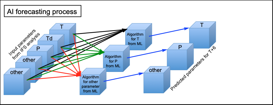
Fig2.2.1-1: Forecasting process using AI for a single parameter for a single step. The algorithm to produce each single parameter uses all the set of input variables. The algorithms relating the observed data to predicted value of each parameter six hours later have been derived by ML. Note: In the diagram "other parameters" include 6hr precipitation and 6hr convective precipitation.

Fig2.2.1-2: Sequence of forecasting processes using AI for all the parameters for a complete 360hr (15day) forecast. Each algorithm to produce each output variable uses all input variables. The algorithms relating observed data to predicted data six hours later have been derived by ML. Note: In the diagram "other parameters" include 6hr precipitation and 6hr convective precipitation.

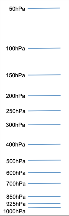
Table2.2.1: The ML machine learning process and the AIFS forecast process use observed and forecast variables and constants. Currently AIFS only uses data at the surface and at standard pressure levels (diagram on the right). Representation of the state of the atmosphere is taken from:
- ERA5 for the ML process.
- the ECMWF operational analysis for the AI forecast process.
Both ML during the training process and AI during the forecast process predict the atmospheric state for six hours in the future.
Highlights and challenges
Strengths of using AI are:
- it gives very rapid results. The observation to output relationships are quite simple and require little processing power at each grid point. As each time step is six hours, few iterations are needed for a forecast. This brings the prospect of very large or very frequent ensembles of AI forecasts.
- it is very cheap to run, because of the simplicity of the relationship program.
- output can be tailored directly to uses other than meteorology (e.g. to health services without any knowledge of medical theory after a ML training process has been performed using health service parameters).
Considerations when using AI are:
- there is no need for comprehensive understanding of physics theory. The relationships are simple to program but at the expense of understanding physically the meteorological effects that are in action.
- the AI process is effectively a "black box" producing results by a process unknown to the user. It requires a good deal of trust in the method though initial results show high effectiveness. The user can have difficulty interpreting or explaining forecast results.
- the ability to interpret the results of AI forecasts ("Interpretability") may be built up with experience; the ability to explain the results of AI forecasts ("Explainability") may be more difficult.
- the set of observed and forecast variables is limited (see Table1).
- post-processing at a given location may require further physical or practical interpretation.
- problems regarding compatibility between programming languages of physical and AI models. This might become a problem where hybrid models are employed (e.g. where transferring data from AI to physical model for post-processing).
- input observations at different times and locations have to be assigned to specific grid points (encoding) and the reverse process to assign forecast values from grid points to specific locations (decoding).
- each forecast variable is independent of the others. They are not interdependent. The forecast wind may not be consistent with the forecast pressure or height gradient.
- vertical velocity is not predicted but could be diagnosed from predicted divergence fields.
- the intensity of smaller-scale features like frontal structures and even in the derived vertical velocity can be in error
Information on issues associated with AIFS Single is given in Known AIFS Single Forecasting Issues
Information on issues associated with AIFS ENS is given in Known AIFS ENS Forecasting Issues
(FUG Associated with Cy49r1)
Overview
Community Forums
Content Tools