Magics' Python interface allows users to visualise Weather Parameter files. These files are a product of ECMWF and are disseminated in BUFR format. A more detailed description of the format can be found in the Meteorological Bulletin M3.1:
http://www.ecmwf.int/sites/default/files/3.1.pdf
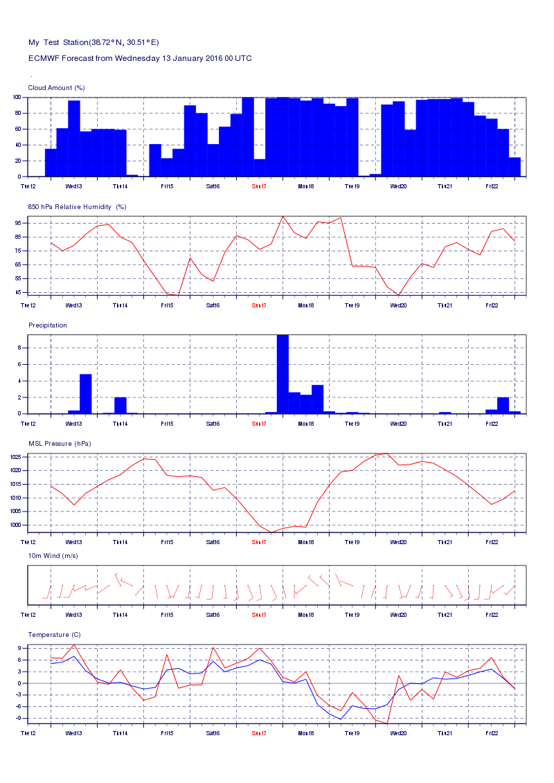
To reproduce what is called a classic metgram as shown below, a small python script needs to be written.
The user can control a few parameters such as:
The PostScript file name for the output
The station position and title. ( Note that the position should be in the BUFR input file)
The list of parameters to be displayed
Step-by-step guide
Example code:
from Magics.macro import *

#Define the output
out = output(
        output_formats=["ps", "png"],
        output_name_first_page_number='off',
        output_name="epsbufr" ,
        super_page_y_length=29.7,
        super_page_x_length=21.,
        )

#Define the layout and projection
# define the cartesian projection
    frame1 = page(
        layout='positional',
        page_x_length= 21.,
        page_y_length= y+3.,
        page_id_line='off',
        page_x_position=0.,
        page_y_position= last
        )
    last = last - y;
    projection = mmap(
        subpage_map_projection='cartesian',
        subpage_x_axis_type='date',
        subpage_x_automatic='on',
        subpage_y_axis_type='regular',
        subpage_y_automatic='on',
        subpage_y_length = suby,
        subpage_y_position = 0.5
        )
    font_size = 0.35
# define horizontal axis
    horizontal = maxis(
        axis_orientation = "horizontal",
        axis_date_type = "days",
        axis_days_label = "both",
        axis_days_label_colour=  "navy",
        axis_days_label_height = font_size,
        axis_grid =  "on",
        axis_grid_colour = "navy",
        axis_grid_line_style= "dash",
        axis_line_colour= "navy",
        axis_minor_tick= "on",
        axis_minor_tick_colour= "navy",
        axis_months_label= "off",
        axis_tick_colour= "navy",
        axis_type =  "date",
        axis_years_label = "off"
        )
# define vertical axis
    vertical = maxis(
        axis_orientation = "vertical",
        axis_grid = "on",
        axis_grid_colour ="navy",
        axis_grid_line_style = "dash",
        axis_grid_reference_level =  0.,
        axis_grid_reference_thickness = 1,
        axis_line =  "on",
        axis_line_colour = "navy",
        axis_tick_colour = "navy",
        axis_tick_label_colour = "navy",
        axis_tick_label_height =  font_size
        )
# Define the input data
    cc_data =    mmetbufr(
                        epsbufr_parameter_title = "Cloud Amount (%)",
                        epsbufr_parameter_descriptor =  20010,
                        epsbufr_information =  "on",
                        epsbufr_input_filename = data["epsbufr_input_filename"],
                        epsbufr_station_latitude = data["epsbufr_station_latitude"],
                        epsbufr_station_longitude = data["epsbufr_station_longitude"],
                        epsbufr_station_name =  "My  Test  Station",
                    )
#Define the graph
    cc_graph = mmetgraph( eps_box_border_thickness = 2,
                          eps_box_width = 1.5,
                          metgram_plot_style = 'bar')
#add a custom title
    cc_text = mtext(
                text_colour =  "navy",
                text_font_size = 0.2,
                text_justification =  "left",
                text_lines =  ["<font size='0.5'> <json_info key='station_info'/></font>",
                    "<font size='0.5'> <json_info key='date'/></font>",
                    "<font size='0.5'> . </font>",
                    "<font size='0.4'> <json_info key='parameter_info'/></font> "]
            )

#Create the plot
    plot(out, frame, projection, horizontal, vertical, cc_data, cc_graph, cc_text, )
You can find a full version of the script metbufr.py and some data.
The script can be executed by typing:
python metbufr.py
The metbufr is expecting a BUFR file as input, and a location to extract from this file. The location is defined by its latitude and longitude, and its name will appear in the title:
mystation  =   mmetbufr(
                        epsbufr_parameter_title = "Cloud Amount (%)",
                        epsbufr_parameter_descriptor =  20010,
                        epsbufr_information =  "on",
                        epsbufr_input_filename = data["epsbufr_input_filename"],
                        epsbufr_station_latitude = data["epsbufr_station_latitude"],
                        epsbufr_station_longitude = data["epsbufr_station_longitude"],
                        epsbufr_station_name =  "My  Test  Station",
                    )
The table below gives an overview of the parameters currently supported:
Table: Metgram parameters
name | BUFR descriptor | scaling | offset | visualisation |
cloud | 20010 | 1 | 0 | blue bar |
humidity | 13003 | 1 | 0 | red curve |
precip | 13011 | 1 | 0 | blue bar |
msl | 10051 | 0.01 | 0 | red curve |
wind | u:11003 v:11004 | 1 | 0 | red flags |
temperature | T2m: 12004 T850:12001 | 1 | -273.15 | T2m as red curveT850 as blue curve |
1 Comment
Stephan Siemen