...
The simulation is defined by the 'fwd_conc' FLEXPART Run icon and the 'rel_volcano' FLEXPART Release icon, respectively. Both these are encompassed in a single macro called 'fw_cond.mv'. For simplicity will use this macro to examine the settings in detail.
The macro starts with defining the release like this:
| Code Block | ||
|---|---|---|
| ||
rel_volcano = flexpart_release( |
...
name : "VOLCANO", |
...
starting_ |
...
date : 0, starting_time : 15, ending_date : 2, ending_time : 12, area : [63.63,-19.6,63.63,-19.6], |
...
top_level : 9000, bottom_level : 1651, particle_count : 10000, masses : 1000000 ) |
This says that the release will happen over a 45 h period between heights 1651 and 10000 m at the location of the volcano and we will release 1000 tons of material in total.
...
The actual simulation is carried out by calling flexpart_run():
| Code Block | ||
|---|---|---|
| ||
#Run flexpart (asynchronous call!) |
...
r = flexpart_run( |
...
output_ |
...
path : "result_fwd_conc", |
...
input_ |
...
path : "../data", |
...
starting_ |
...
date : 20120517, starting_time : 12, ending_date : 20120519, ending_time : 12, output_field_type: "concentration", |
...
output_ |
...
flux : "on", |
...
output_ |
...
trajectory : "on", |
...
output_ |
...
area : [40,-25,66,10], |
...
output_ |
...
grid : [0.25,0.25], |
...
output_ |
...
levels : [500,1000,2000,3000,4000,5000,7500,10000,15000], |
...
release_species : |
...
8, receptors : "on", |
...
receptor_ |
...
names : ["rec1","rec2"], |
...
receptor_ |
...
latitudes : [60,56.9], |
...
receptor_longitudes : |
...
[6.43,-3.5], |
...
releases : rel_volcano ) print(r) |
Here we defined both the input and output path and specified the simulation period, the output grid and levels as well. We also told FLEXPART to generate gridded concentration fields and plume trajectories on output..
| Info |
|---|
The actual species that will be released is defined as an integer number (for details about using the species see here). With the default species settings number 8 stands for SO2. |
...
If we run this macro (or alternatively right-click execute the FLEXPART Run icon) the results (after a minute or so) will be available in folder 'result_fw_conc' . The computations were actually taken place in a temporary folder then metview copied the results to the output folder. If we open this older we will see two files there:
...
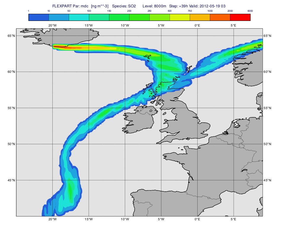
The macro to visualise the concentration fields on a given level is 'plot_level.mv'.
First, we define the level (8000 m) and the parameter ("mdc") we want to plot. Then we call mvl_flexpart_read_hl() to filter the data into a fieldset.
| Code Block |
|---|
dIn="result_fwd_conc/" |
...
inFile= |
...
dIn & "conc_s001.grib" |
...
lev=8000 |
...
par="mdc" |
...
#Read fields on the given height level g=mvl_flexpart_read_hl(inFile,par,lev,-1,-1) |
Next, we define the contouring definition. The units we used here are ng m**-3 because for parameter "mdc" the native units (kg m**-3) are automatically scaled by the plotting library (see details about the this scaling for various FLEXPART GRIB fields here.
| Code Block | ||
|---|---|---|
| ||
#The contour levels |
...
cont_list=[1,10,50,100,150,200,250,500,750,1000,2000,6000] |
...
#Define contour shading conc_shade = mcont( |
...
legend : "on", |
...
contour : "off", |
...
contour_level_selection_ |
...
type : "level_list", |
...
contour_level_ |
...
list : cont_list, |
...
contour_ |
...
label : "off", |
...
contour_ |
...
shade : "on", |
...
contour_shade_ |
...
method : "area_fill", |
...
contour_shade_max_level_ |
...
colour : "red", |
...
contour_shade_min_level_ |
...
colour : "RGB(0.14,0.37,0.86)", |
...
contour_shade_colour_ |
...
direction : "clockwise", |
...
contour_method: "linear" |
...
) |
Next, we build the title with mvl_flexpart_title(). Please note that we need to explicitly specify the plotting units!
| Code Block | ||
|---|---|---|
| ||
title=mvl_flexpart_title(g,0.3,"ng m**-3") |
Finally we define the view with the map:
| Code Block | ||||
|---|---|---|---|---|
|
...
| |||
#Define coastlines
coast_grey = mcoast(
	map_coastline_thickness	:	2,
	map_coastline_land_shade	:	"on",
	map_coastline_land_shade_colour	:	"grey",
	map_coastline_sea_shade	:	"on",
	map_coastline_sea_shade_colour	:	"RGB(0.89,0.89,0.89)",
	map_boundaries	:	"on",
	map_boundaries_colour	:	"black",
	map_grid_latitude_increment	:	5,
	map_grid_longitude_increment	:	5
	)

#Define geo view
view = geoview(
	map_area_definition	:	"corners",
	area	:	[40,-25,66,9],
	coastlines: coast_grey
) |
and generate the plot:
| Code Block | ||
|---|---|---|
| ||
plot(view,g,conc_shade,title) |
Having run the we get a plot like this (after navigating to step 39h):