This tutorial demonstrates how to run a forward simulation with FLEXPART and how to visualise the results in various ways.
| Expand |
|---|
| title | Click here to see the preparation instructions ... |
|---|
|
| Excerpt Include |
|---|
| Using FLEXPART with Metview |
|---|
| Using FLEXPART with Metview |
|---|
|
|
| Table of Contents |
|---|
| exclude | Preparations|The input data |
|---|
|
Please enter folder 'fwd' to start working.
Running the simulation
We will simulate a volcano eruption by releasing some SO2 from the Icelandic volcano Eyjafjallajökull.
The simulation itself is defined by the 'fwd_conc' FLEXPART Run icon and the 'rel_volcano' FLEXPART Release icon, respectively. Both these are encompassed in a single macro called 'fw_cond.mv'. For simplicity will use this macro to examine the settings in detail.
The macro starts with defining the release like this:
| Code Block |
|---|
|
rel_volcano = flexpart_release(
    name            :   "VOLCANO",
    starting_date   :   0,
    starting_time   :   15,
    ending_date     :   2,
    ending_time     :   12,
    area            :   [63.63,-19.6,63.63,-19.6],
    top_level       :   9000,
    bottom_level    :   1651,
    particle_count  :   10000,
    masses          :   1000000
) |
This says that the release will happen over a 45 h period between heights 1651 and 10000 m at the location of the volcano and we will release 1000 tons of material in total.
| Info |
|---|
Please note that - the species is not defined here (will be defined in
flexpart_run()) - we used dates relative to the starting date of the simulation (see also in
flexpart_run())
|
The actual simulation is carried out by calling flexpart_run():
| Code Block |
|---|
|
#Run flexpart (asynchronous call!)

r = flexpart_run(
    output_path     	:   "result_fwd_conc",
    input_path      	:   "../data",
    starting_date   	:   20120517,
    starting_time   	:   12,
    ending_date     	:   20120519,
    ending_time     	:   12,
    output_field_type	:   "concentration",
    output_flux     	:   "on",
    output_trajectory   :   "on",
    output_area     	:   [40,-25,66,10],
    output_grid     	:   [0.25,0.25],
    output_levels   	:   [500,1000,2000,3000,4000,5000,7500,10000,15000],
    release_species 	:   8,
    receptors       	:   "on",
    receptor_names  	:   ["rec1","rec2"],
    receptor_latitudes  :   [60,56.9],
    receptor_longitudes :   [6.43,-3.5],
    releases        	:   rel_volcano
    )

print(r) |
Here we defined both the input and output path and specified the simulation period, the output grid and levels as well. We also told FLEXPART to generate gridded concentration fields and plume trajectories on output..
| Info |
|---|
The actual species that will be released is defined as an integer number (for details about using the species see here). With the default species settings number 8 stands for SO2. |
If we run this macro (or alternatively right-click execute the FLEXPART Run icon) the results (after a minute or so) will be available in folder 'result_fw_conc' . The computations were actually taken place in a temporary folder then metview copied the results to the output folder. If we open this older we will see two files there:
- conc_s001.grib is GRIB file containing the gridded concentration fields
- tr_r1.csv is CSV file containing the plume trajectories
| Info |
|---|
Please note that these are not the original outputs form FLEXTRA but were converted to formats more suitable for use in Metview. For details about the FLEXPART outputs please click here. |
Visualising gridded fields
To plot a particular parameter and level we need to filter the desired dataset from the resulting FLEXPART output file. Unfortunately, Metview's Grib Filter icon cannot handle these files (partly due to the local GRIB definition they use) so we need to use other means to cope with this task. For this reason and also to make FLEXPART output handling easier a set of Metview Macro Library Functions were developed. We will heavily use these functions in the examples below.
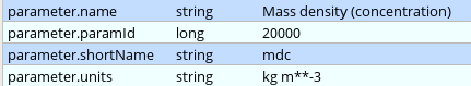
Inspecting the FLEXPART GRIB file
Before seeing the macro code to generate the plot we inspect the file itself we wanted to plot. Double-click on the 'conc_s001.grib' GRIB icon' in folder 'result_fw_conc' to start up the Grib Examiner. We can see that this file only contains "mdc" (=Mass density concentration) fields. We can find out further details about this parameter by setting the Dump mode to Namespace and Namespace to Parameter:
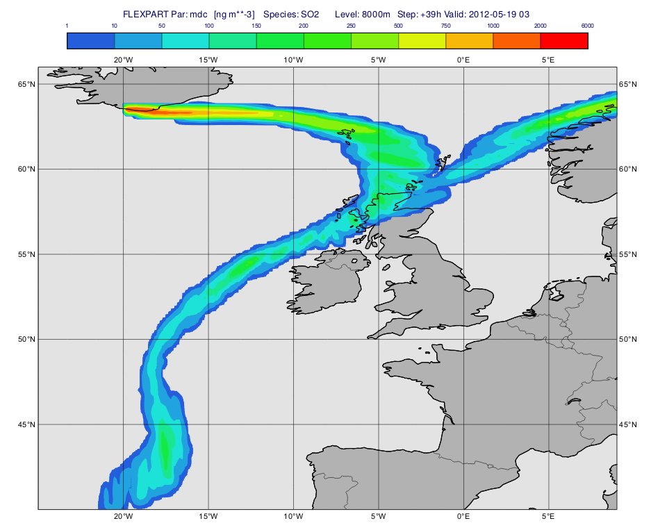
Generating the plot
The macro to visualise the concentration fields on a given level is 'plot_level.mv'.
First, we define the level (8000 m) and the parameter ("mdc") we want to plot. Then we call the Macro Library Function mvl_flexpart_read_hl() to extract the data to plot.
| Code Block |
|---|
dIn="result_fwd_conc/"
inFile=dIn  & "conc_s001.grib"
lev=8000
par="mdc"

#Read fields on the given height level
g=mvl_flexpart_read_hl(inFile,par,lev,-1,1) |
Next, we define the contouring definition. The units we used here are ng m**-3 because for parameter "mdc" the native units (kg m**-3) are automatically scaled by the plotting library (see details about the this scaling for various FLEXPART GRIB fields here.
| Code Block |
|---|
|
#The contour levels
cont_list=[1,10,50,100,150,200,250,500,750,1000,2000,6000]

#Define contour shading
conc_shade = mcont(
    legend  						:   "on",
    contour 						:   "off",
    contour_level_selection_type	:   "level_list",
    contour_level_list  			: 	cont_list,
    contour_label   				:   "off",
    contour_shade   				:   "on",
    contour_shade_method    		:   "area_fill",
    contour_shade_max_level_colour  :   "red",
    contour_shade_min_level_colour  :   "RGB(0.14,0.37,0.86)",
    contour_shade_colour_direction  :   "clockwise",
    contour_method					: 	"linear"
) |
Next, we build the title with mvl_flexpart_title(). Please note that we need to explicitly specify the plotting units!
| Code Block |
|---|
|
title=mvl_flexpart_title(g,0.3,"ng m**-3") |
Finally we define the view with the map:
| Code Block |
|---|
| language | py |
|---|
| title | Defining the map view |
|---|
| collapse | true |
|---|
|
#Define coastlines
coast_grey = mcoast(
	map_coastline_thickness			:	2,
	map_coastline_land_shade		:	"on",
	map_coastline_land_shade_colour	:	"grey",
	map_coastline_sea_shade			:	"on",
	map_coastline_sea_shade_colour	:	"RGB(0.89,0.89,0.89)",
	map_boundaries					:	"on",
	map_boundaries_colour			:	"black",
	map_grid_latitude_increment		:	5,
	map_grid_longitude_increment	:	5
	)

#Define geo view
view = geoview(
	map_area_definition	:	"corners",
	area				:	[40,-25,66,9],
	coastlines			: coast_grey
) |
and generate the plot:
| Code Block |
|---|
|
plot(view,g,conc_shade,title) |
Having run the macro we will get a plot like this (after navigating to step 39h):
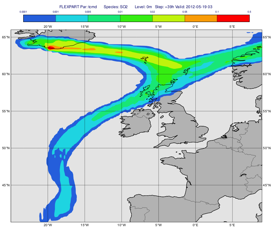
Computing and plotting total column mass
Using the same FLEXPART output as above we will compute and plot the total column integrated mass. The macro to use is 'plot_total.mv'.
First, we call mvl_flexpart_total_column() to perform the computations. The result is a fieldset containing "tcmd" fields with units of "kg m**-2".
| Code Block |
|---|
dIn="result_fwd_conc/"
inFile=dIn  & "conc_s001.grib"

#Compute the total column integrated mass
g=mvl_flexpart_total_column(inFile,1)
|
Next, we define the contouring. The "tcmd" fields are automatically scaled into "ng m**-2" for contouring (see here for details) but with the current value range it is better to use "g m**-2" units. To achieve it we simply multiply the "tcmd" fieldset with 1000:
The contour definition itself goes like this:
| Code Block |
|---|
|
cont_list=[0.0001,0.001,0.005,0.01,0.02,0.05,0.1,0.5]

#Define contour shading
conc_shade = mcont(
	legend							:	"on",
	contour							:	"off",
	contour_level_selection_type	:	"level_list",
	contour_level_list  			:   cont_list,
	contour_label					:	"off",
	contour_shade					:	"on",
	contour_shade_method			:	"area_fill",
	contour_shade_max_level_colour	:	"red",
	contour_shade_min_level_colour	:	"RGB(0.14,0.37,0.86)",
	contour_shade_colour_direction	:	"clockwise",
    contour_method					: 	"linear",
    grib_scaling_of_derived_fields	: 	"off"
    )
|
Please note that by multiplying our fieldset by 1000 it became a derived fieldset. Since we do not want the automatic contour scaling to happen we need to set the contouring parameter grib_scaling_of_derived_fields to "off".
Next, we build the title with mvl_flexpart_title(). Please note that we need to explicitly specify the plotting units!
| Code Block |
|---|
|
title=mvl_flexpart_title(g,0.3,"g m**-2") |
Finally we define the view with the map in the same way as above and generate the plot:
| Code Block |
|---|
|
plot(view,g,conc_shade,title) |
Having run the macro we will get a plot like this (after navigating to step 39h):
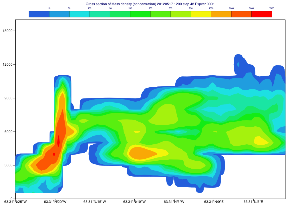
Plotting a vertical cross section
Using the same FLEXPART output as above we will plot a vertical cross section. The macro to use is 'plot_xs.mv'.
First, we define the parameter and time step for the cross section then call mvl_flexpart_read_hl() to extract the data. The result is a fieldset with units of "kg m**-3" that we need to explicitly convert to "ng m**-3" units for plotting since the automatic units scaling only works for map based plots.
| Code Block |
|---|
|
#Define level, parameter and step
lev=-1 #all levels
par="mdc"
step=48

#Get fields for all levels for a given step
g=mvl_flexpart_read_hl(inFile,par,lev,step,1)

#Scale into ng/m3 units
g=g*1000000000000
|
Next, we define the cross section view:
| Code Block |
|---|
|
xs_view = mxsectview(
	bottom_level	:	0,
	top_level	:	16000,
	line	:	[63.31,-25,63.31,9]
	)
|
Then, we define the contouring:
| Code Block |
|---|
| language | py |
|---|
| title | Define contouring |
|---|
| collapse | true |
|---|
|
#The contour levels
cont_list=[1,10,50,100,150,200,250,500,750,1000,2000,5000,7000]

#Define contour shading
conc_shade = mcont(
	legend	:	"on",
	contour	:	"off",
	contour_level_selection_type	:	"level_list",
	contour_level_list  : cont_list,
	contour_label	:	"off",
	contour_shade	:	"on",
	contour_shade_method	:	"area_fill",
	contour_shade_max_level_colour	:	"red",
	contour_shade_min_level_colour	:	"RGB(0.14,0.37,0.86)",
	contour_shade_colour_direction	:	"clockwise",
    contour_method: "linear"
) |
and finally generate the plot:
| Code Block |
|---|
|
plot(xs_view,g,conc_shade) |
Having run the macro we will get a plot like this: