Check the initial conditions
The initial conditions are available under the master (troifs0) training account. You do not need to copy them, but you can check the content of the folder as well as the files.
| Code Block |
|---|
troifs1@cca-login4:/perm/ectrain/troifs1> ls -ltr /perm/ectrain/troifs0/user-cray/oifs40r1/data/input/
|
| Panel |
|---|
| borderColor | #cccccc |
|---|
| borderWidth | 1 |
|---|
| borderStyle | solid |
|---|
| title | Input data |
|---|
|
| HTML |
|---|
<table>
<tr>
<td valign="top"><p style="line-height: 1.2;"><strong>File name</strong></p></td>
<td valign="top"><p style="line-height: 1.2;"> </p></td>
<td valign="top"><p style="line-height: 1.2;"><strong>Description</strong></p></td>
<td valign="top" align="right"><p style="line-height: 1.2;"><strong>Size</strong></p></td>
</tr>
<tr>
<tr>
<td valign="top"><p style="font-family: Monospace; line-height: 1.2;">2015120300/ICMCLgs0cINIT</p></td>
<td valign="top"><p style="font-family: Monospace; line-height: 1.2;">: </p></td>
<td valign="top"><p style="font-family: Monospace; line-height: 1.2;">input file containing surface and soil information (albedo, soil temperature etc.)</p></td>
<td valign="top" align="right"><p style="font-family: Monospace; line-height: 1.2;">9.3 MB</p></td>
</tr>
<tr>
<td valign="top"><p style="font-family: Monospace; line-height: 1.2;"> 2015120300/ICMGGgs0cINIT</p></td>
<td valign="top"><p style="font-family: Monospace; line-height: 1.2;">: </p></td>
<td valign="top"><p style="font-family: Monospace; line-height: 1.2;">input file containing gridpoint surface initial data</p></td>
<td valign="top" align="right"><p style="font-family: Monospace; line-height: 1.2;">7 MB</p></td>
</tr>
<tr>
<td valign="top"><p style="font-family: Monospace; line-height: 1.2;"> 2015120300/ICMSHgs0cINIT</p></td>
<td valign="top"><p style="font-family: Monospace; line-height: 1.2;">: </p></td>
<td valign="top"><p style="font-family: Monospace; line-height: 1.2;">input file containing initial data for the prognostic variables in spectral representation</p></td>
<td valign="top" align="right"><p style="font-family: Monospace; line-height: 1.2;">35 MB</p></td>
</tr>
<tr>
<td valign="top"><p style="font-family: Monospace; line-height: 1.2;"> 2015120300/ICMGGgs0cINIUA</p></td>
<td valign="top"><p style="font-family: Monospace; line-height: 1.2;">: </p></td>
<td valign="top"><p style="font-family: Monospace; line-height: 1.2;">input file containing initial data for the prognostic variables in gridpoint representation</p></td>
<td valign="top" align="right"><p style="font-family: Monospace; line-height: 1.2;"> 101 MB</p></td>
</tr>
<tr>
<td valign="top"><p style="font-family: Monospace; line-height: 1.2;"> 2015120300/wam_grid_tables</p></td>
<td valign="top"><p style="font-family: Monospace; line-height: 1.2;">: </p></td>
<td valign="top"><p style="font-family: Monospace; line-height: 1.2;">model grid and tables for the wave model</p></td>
<td valign="top" align="right"><p style="font-family: Monospace; line-height: 1.2;">52 MB</p></td>
</tr>
<tr>
<td valign="top"><p style="font-family: Monospace; line-height: 1.2;"> 2015120300/wam_subgrid_0</p></td>
<td valign="top"><p style="font-family: Monospace; line-height: 1.2;">: </p></td>
<td valign="top"><p style="font-family: Monospace; line-height: 1.2;">information for model advection, including sub-grid parametrisation for the wave model</p></td>
<td valign="top" align="right"><p style="font-family: Monospace; line-height: 1.2;">12 MB</p></td>
</tr>
<tr>
<td valign="top"><p style="font-family: Monospace; line-height: 1.2;"> 2015120300/wam_subgrid_1</p></td>
<td valign="top"><p style="font-family: Monospace; line-height: 1.2;">: </p></td>
<td valign="top"><p style="font-family: Monospace; line-height: 1.2;">information for model advection, including sub-grid parametrisation for the wave model</p></td>
<td valign="top" align="right"><p style="font-family: Monospace; line-height: 1.2;">25 MB</p></td>
</tr>
<tr>
<td valign="top"><p style="font-family: Monospace; line-height: 1.2;"> 2015120300/wam_subgrid_2</p></td>
<td valign="top"><p style="font-family: Monospace; line-height: 1.2;">: </p></td>
<td valign="top"><p style="font-family: Monospace; line-height: 1.2;">information for model advection, including sub-grid parametrisation for the wave model</p></td>
<td valign="top" align="right"><p style="font-family: Monospace; line-height: 1.2;">25 MB</p></td>
</tr>
<tr>
<td valign="top"><p style="font-family: Monospace; line-height: 1.2;"> 2015120300/cdwavein</p></td>
<td valign="top"><p style="font-family: Monospace; line-height: 1.2;">: </p></td>
<td valign="top"><p style="font-family: Monospace; line-height: 1.2;">initial value of drag coefficient for the wave model</p></td>
<td valign="top" align="right"><p style="font-family: Monospace; line-height: 1.2;">63 KB</p></td>
</tr>
<tr>
<td valign="top"><p style="font-family: Monospace; line-height: 1.2;"> 2015120300/specwavein</p></td>
<td valign="top"><p style="font-family: Monospace; line-height: 1.2;">: </p></td>
<td valign="top"><p style="font-family: Monospace; line-height: 1.2;">initial wave spectra for the wave model</p></td>
<td valign="top" align="right"><p style="font-family: Monospace; line-height: 1.2;">7.6 MB</p></td>
</tr>
<tr>
<td valign="top"><p style="font-family: Monospace; line-height: 1.2;"> 2015120300/uwavein</p></td>
<td valign="top"><p style="font-family: Monospace; line-height: 1.2;">: </p></td>
<td valign="top"><p style="font-family: Monospace; line-height: 1.2;">initial value of wind speed for the wave model</p></td>
<td valign="top" align="right"><p style="font-family: Monospace; line-height: 1.2;">63 KB</p></td>
</tr>
<tr>
<td valign="top"><p style="font-family: Monospace; line-height: 1.2;"> 2015120300/sfcwindin</p></td>
<td valign="top"><p style="font-family: Monospace; line-height: 1.2;">: </p></td>
<td valign="top"><p style="font-family: Monospace; line-height: 1.2;">initial value of 10-metre horizontal wind components and sea ice fraction for the wave model</p></td>
<td valign="top" align="right"><p style="font-family: Monospace; line-height: 1.2;">2.2 MB</p></td>
</tr>
</table> |
|
The initial conditions are GRIB files, you can read their content using ecCodes commands, e.g.:
| Code Block |
|---|
troifs1@cca-login4:/perm/ectrain/troifs1> grib_ls /perm/ectrain/troifs0/user-cray/oifs40r1/data/input/ICMSHgs0cINIT |
Edit the namelist
The namelist files control the necessary experiment settings (e.g., time step, experiment ID) as well as the post-processing. The namelists are in the nam directory, go there and open the namelistfc file using a text editor, e.g.:
| Code Block |
|---|
troifs1@cca-login4:/perm/ectrain/troifs1> cd oifs40r1/nam
troifs1@cca-login4:/perm/ectrain/troifs1/oifs40r1/nam> gvim namelistfc
|
The most important namelist elements are listed below with their explanation:
| Panel |
|---|
| borderColor | #cccccc |
|---|
| borderWidth | 1 |
|---|
| borderStyle | solid |
|---|
| title | Sample namelist |
|---|
|
&NAMDYN ! Name of the namelist group
TSTEP=2700.0, ! Time step in seconds
/ ! End of the namelist group
&NAMFPG
NFPLEV=91, ! Number of vertical levels
NFPMAX=255, ! Spectral truncation
/
&NAMCT0
CNMEXP="gs0c",           ! Experiment ID
 NFRPOS=4,                ! Output frequency of the 'history' files  in time steps (i.e. here 3 hours)
 NFRHIS=4,                 ! Output frequency of the model variables in time steps (i.e. here 3 hours)
/
&NAMFPC
! Pressure level outputs: number of fields (NFP3DFP), GRIB field codes (MFP3DFP) and pressure levels in Pascals (RFP3P)
NFP3DFP=9,
 MFP3DFP(:)=129,130,135,138,155,157,133,131,132,
 RFP3P(:)=100000.0,92500.0,85000.0,70000.0,50000.0,40000.0,30000.0,25000.0,20000.0,15000.0,10000.0,7000.0,5000.0,3000.0,2000.0,1000.0,700.0,500.0,300.0,200.0,100.0,
  ! Saving spectral orography (geopotential), surface pressure (logarithm of surface pressure) needed for post-processing
NFP2DF=2,
MFP2DF(:)=129,152,
 ! Physics output: number of fields (NFPPHY) and GRIB field codes (MFPPHY)
NFPPHY=89,
 MFPPHY(:)=31,32,33,34,35,36,37,38,39,40,41,42,44,45,49,50,57,58,59,78,79,129,136,137,139,141,142,143,144,145,146,147,148,151,159,164,165,166,167,168,169,170,172,175,176,177,178,179,180,181,182,183,186,187,188,189,195,196,197,198,201,202,205,206,208,209,210,211,235,236,238,243,244,245,229,230,231,232,213,212,8,9,228089,228090,228001,260121,260123,228129,228130,
/
&NAMFPD
NLAT=256,                   !  Number of latitudes on the corresponding Gaussian grid
NLON=512,                   ! Number of longitudes on the corresponding Gaussian grid
/
|
In the evaluation, we will investigate the following variables:
| HTML |
|---|
<p>These variables have to be included in the namelist among the post-processing variables (see the code numbers and levels highlighted with <b>bold</b> characters in the box above). More information about the namelist settings and GRIB field codes of different parameters can be found in the <b><a href="https://confluence.ecmwf.int/display/OIFS/How-to+articles" target="_blank">OpenIFS how-to articles</a></b>: <a href="https://confluence.ecmwf.int/display/OIFS/How+to+control+OpenIFS+output" target="_blank">How to control OpenIFS output</a>.</p>
|
Submit the experiment
The experiment will be executed by submission of the job_desmond file.
| Expand |
|---|
| title | Click here to see the steps this programme does. |
|---|
|
Clean the working directory where your experiment will run: | Code Block |
|---|
cd $RUNDIR
/bin/rm -R ouput1 ICM* ifsdata rtables *l_2 wam* *in fort.* master.exe MPP* |
Copy or link the initial conditions from the input directory to your working directory: | Code Block |
|---|
ln -sf ${INPUTDIR}/ICM* .
ln -sf ${INPUTDIR}/wam* .
ln -sf ${INPUTDIR}/*in . |
- Set the necessary environment variables:
- OIFS_GRIB_DIR: folder of ecCodes
- OIFS_DATA_DIR: folder of climate data called ifsdata
Copy the namelists to your working directory: | Code Block |
|---|
cp -sf ${NAMDIR}/namelistfc fort.4
ln -sf ${NAMDIR}/wam_namelist .
ln -sf ${NAMDIR}/wam_namelist_coupled_000 . |
Run the model using the oifs_run.sh script. To run the script the experiment ID, the executable file (named master.exe) and the forecast length have to be specified and one can set the spectral truncation as well as the timestep here: | Code Block |
|---|
# oifs_run.sh -e${expID} -m${executable} -r${RESOUTION} -f${SCLENGTH} -s${TSTEP}
${JOBDIR}/oifs_run.sh -egs0c -m${BINDIR}/master.exe -r255 -fh54 -s2700. > out 2>err |
With these settings you run a 54-hour forecast (-fh54), where JOBDIR and BINDIR are the location of the oifs_run.sh script and the master.exe OpenIFS executable, respectively.
Before the model run begins, the oifs_run.sh script checks the inputs and ensures that the necessary climate data on the corresponding resolution are also available in your working directory. Move the output files to the output directory: | Code Block |
|---|
mv ${RUNDIR}/ICMGG${OIFS_EXPID}+* ${OUTPUTDIR}/
mv ${RUNDIR}/ICMSH${OIFS_EXPID}+* ${OUTPUTDIR}/ |
|
We submit the job with the qsub command:
| Code Block |
|---|
troifs1@cca-login4:/perm/ectrain/troifs1/oifs40r1/nam> cd ../job
troifs1@cca-login4:/perm/ectrain/troifs1/oifs40r1/job> qsub job_desmond |
After the job is submitted, you can check its status with the qstat command:
| Code Block |
|---|
troifs1@cca-login4:/perm/ectrain/troifs1/oifs40r1/job> qstat -u $USER

ccapar:
                                                            Req'd  Req'd   Elap
Job ID          Username Queue    Jobname    SessID NDS TSK Memory Time  S Time
--------------- -------- -------- ---------- ------ --- --- ------ ----- - -----
1875659.ccapar troifs1 np troifs1 50171 3 72 241gb 30:00 R 00:10 |
if you see 'R' under 'S' in the output message, it means that your job is running. If it is in 'Q' status, it is still queueing. If you have not received any message, it means either your job successfully finished or failed.
When OpenIFS starts to run, you will see the following content in your working directory:
| Code Block |
|---|
master.exe        fort.4                                               # executable and namelist
wam_namelist      wam_namelist_coupled_000						       # namelists for the wave model
ICMGGgs0cINIUA    ICMCLgs0cINIT    ICMSHgs0cINIT     ICMGGgs0cINIT     # initial conditions
cdwavein          sfcwindin        specwavein        uwavein		   # wave model initial conditions
wam_grid_tables   wam_subgrid_0    wam_subgrid_1     wam_subgrid_2     # wave model files
ifsdata           rtables          255l_2						       # climate data
ncf927            ifs.stat         NODE.001_01                         # text output (log) files
out               err                                                  # output and error files from the model run
ICMGGgs0c+000000 ICMSHgs0c+000000 ICMGGgs0c+000003 ICMSHgs0c+000003 # output files for the first two steps |
The running time of the job is around 10 minutes, the outputs (i.e. the ICM* files) are continuously generated. If your job failed, you find more information about the reason in the NODE.001_01 and the err files. We suggest starting their inspection at the end of the file.
| HTML |
|---|
For more instructions and details about running the model, please visit the related <a href="https://confluence.ecmwf.int/display/OIFS/5.6+Acceptance+testing+OpenIFS+after+installation" target="_blank">page</a> in the <a href="https://confluence.ecmwf.int/display/OIFS/OpenIFS+User+Guides" target="_blank">OpenIFS User Guides</a>. |
Post-processing the model outputs
After the job run is completed, the outputs are split into 2 files (located in the working directory): ICMGG* files are for the gridpoint fields and ICMSH* files are for the spectral ones. The two kinds of files should include all the necessary variables set in the namelist. However, before visualization of the results, some steps are still needed. The Metview macros prepared for visualization of experiment results require the meteorological variables in GRIB format separated by variables and days with the appropriate names.
Go to the folder where your output files are saved. The 2-metre temperature, the precipitation, the mean sea level pressure and the wind gust are expected in gridpoint representation. They are prepared from the ICMGG* outputs with the next operations:
| Code Block |
|---|
troifs1@cca-login4:/perm/ectrain/troifs1/oifs40r1/job> cd ../data/output/
troifs1@cca-login4:/perm/.../output> expID=gs0c; date=20151204
troifs1@cca-login4:/perm/.../output> steps="00 03 06 09 12 15 18 21 24 27 30 33 36 39 42 45 48 51 54" # every 3 hours from 0 UTC on 4 December to 0 UTC on 6 December
troifs1@cca-login4:/perm/.../output> for step in ${steps}
   do
      grib_copy -w shortName=2t   ICMGG${expID}+0000${step} t2_${date}_${step}.grib    #to get the 2-metre temperature
      grib_copy -w shortName=msl  ICMGG${expID}+0000${step} mslp_${date}_${step}.grib  #to get the mean sea level pressure
      grib_copy -w shortName=10fg ICMGG${expID}+0000${step} gust_${date}_${step}.grib  #to get the 10-metre wind gust
done |
| Note |
|---|
Please do not forget to press Enter after the last command. |
For precipitation, both the convective and large-scale precipitation components have to be gathered in the same file:
| Code Block |
|---|
troifs1@cca-login4:/perm/.../output> expID=gs0c; date=20151204
troifs1@cca-login4:/perm/.../output> steps="00 03 06 09 12 15 18 21 24 27 30 33 36 39 42 45 48 51 54" # every 3 hours from 0 UTC on 4 December to 0 UTC on 6 December
troifs1@cca-login4:/perm/.../output> for step in ${steps}
   do
      grib_copy -w shortName=lsp/cp ICMGG${expID}+0000${step} p_${date}_${step}.grib
done |
The pressure level data are required in spectral representation. They are prepared from the ICMSH* outputs with the next operations:
| Code Block |
|---|
troifs1@cca-login4:/perm/.../output> expID=gs0c; date=20151204
troifs1@cca-login4:/perm/.../output> steps="00 03 06 09 12 15 18 21 24 27 30 33 36 39 42 45 48 51 54" # every 3 hours from 0 UTC on 4 December to 0 UTC on 6 December
troifs1@cca-login4:/perm/.../output> for step in ${steps}
   do
      grib_copy -w shortName=t,level=850 ICMSH${expID}+0000${step} t850_${date}_${step}.grib  #to get the temperature at 850 hPa
      grib_copy -w shortName=r,level=700 ICMSH${expID}+0000${step} q700_${date}_${step}.grib  #to get the relative humidity at 700 hPa
      grib_copy -w shortName=z,level=500 ICMSH${expID}+0000${step} z500_${date}_${step}.grib  #to get the geopotential at 500 hPa
done |
For wind, both the u and v components have to be collected in the same file:
| Code Block |
|---|
troifs1@cca-login4:/perm/.../output> expID=gs0c; date=20151204
troifs1@cca-login4:/perm/.../output> steps="00 03 06 09 12 15 18 21 24 27 30 33 36 39 42 45 48 51 54" # every 3 hours from 0 UTC on 4 December to 0 UTC on 6 December
troifs1@cca-login4:/perm/.../output> for step in ${steps}
   do
      grib_copy -w shortName=u/v,level=250 ICMSH${expID}+0000${step} u250_${date}_${step}.grib  #to get the u and v components at 250 hPa
      grib_copy -w shortName=u/v,level=100 ICMSH${expID}+0000${step} u100_${date}_${step}.grib  #to get the u and v components at 100 hPa
done |
After these operations, the timesteps belonging to the same days have to be merged into a common file and the concatenated file has to be moved to the input directory of the Metview visualization:
| Code Block |
|---|
troifs1@cca-login4:/perm/.../output> expID=gs0c; date=20151204
troifs1@cca-login4:/perm/.../output> variables="t2 mslp gust p t850 q700 z500 u250 u100"
troifs1@cca-login4:/perm/.../output> for variable in ${variables}
   do
      cat ${variable}_${date}_*.grib > ${variable}_${date}.grib
done |
If you are confident that all the necessary files are generated, you can remove the temporary files from the directory:
| Code Block |
|---|
troifs1@cca-login4:/perm/.../output> expID=gs0c; date=20151204
troifs1@cca-login4:/perm/.../output> variables="t2 mslp gust p t850 q700 z500 u250 u100"
troifs1@cca-login4:/perm/.../output> for variable in ${variables}
   do
      /bin/rm ${variable}_${date}_*.grib
done |
At the end you have to have the following files:
| Code Block |
|---|
troifs1@cca-login4:/perm/.../output> ls *grib
gust_20151204.grib  # wind gust
p_20151204.grib     # precipitation
t2_20151204.grib    # 2-metre temperature
mslp_20151204.grib  # mean sea level pressure
q700_20151204.grib  # 700 hPa relative humidity
t850_20151204.grib  # 850 hPa temperature
u100_20151204.grib	# 100 hPa wind
u250_20151204.grib  # 250 hPa wind
z500_20151204.grib  # 500 hPa wind
|
Create directory structure for visualization on the cluster of the University of Reading
Open a terminal window on the cluster of the University of Reading (please do not forget to login with ssh -X username@racc.rdg.ac.uk). The tutorial explains the operations on the cluster using the tswx18101 account, you should replace it with your own user account. Let us assume that the current directory is the ${HOME} directory. The necessary folders are automatically created by the next command:
| Code Block |
|---|
[swx18101@racc-login-0-4 ~] . /home/users/swx18100/Monday_training/Desmond_casestudy/create_environment |
| Note |
|---|
Please note that this command can be started from any directory and in this case you should not change the swx18100 user ID in the path. |
This command creates the following structure in your home directory:
| Code Block |
|---|
|
[swx18101@racc-login-0-4 ~] cd
[swx18101@racc-login-0-4 ~] find .
.
./Monday_trainig								# Directory for training exercises on Monday
./Monday_trainig/Desmond_casestudy				# Directory for exercise with Desmond case study
./Monday_trainig/Desmond_casestudy/data			# Directory for input data
./Monday_trainig/Desmond_casestudy/data/forecast
./Monday_trainig/Desmond_casestudy/data/forecast/gs0c
./Monday_trainig/Desmond_casestudy/data/reference
./Monday_trainig/Desmond_casestudy/macros		# Directory for Metview macros
./Monday_trainig/Desmond_casestudy/macros/plot_forecastrun.mv
./Monday_trainig/Desmond_casestudy/macros/plot_ERA5.mv
./Monday_trainig/Desmond_casestudy/figures		# Directory for figures to save
./Monday_trainig/Desmond_casestudy/definitions	# Directory for some visual definitions
./Monday_trainig/Desmond_casestudy/definitions/base_title.mv
./Monday_trainig/Desmond_casestudy/definitions/base_legend.mv
./Monday_trainig/Desmond_casestudy/definitions/base_layout.mv
./Monday_trainig/Desmond_casestudy/definitions/visdef
./Monday_trainig/Desmond_casestudy/definitions/diff_range
./metview/Desmond_casestudy # Link to casestudy folder in metview directory |
Transfer the forecast data to the cluster of the University of Reading
Navigate to the directory prepared for the forecast data in the folder of the Desmond casestudy:
| Code Block |
|---|
[swx18101@racc-login-0-4 ~]$ cd Monday_training/Desmond_casestudy/data/forecast/gs0c
[swx18101@racc-login-0-4 gs0c]$ sftp -r troifs1@ecaccess.ecmwf.int
cd ECHOST/cca/perm/ectrain/troifs1/oifs40r1/data/output
mget *grib
bye
|
Download the re-analysis data
| HTML |
|---|
<p>As reference data, we use <b>ERA5 re-analyses</b>. ERA5 datasets are public and available in the ECMWF MARS (Meteorological Archival and Retrieval System). Re-analyses are created by optimal combination of available observational information and short-range numerical weather predictions using data assimilation techniques. They provide the most comprehensive description of the past and current states of the 3-dimensional atmosphere or the Earth system.

<p><b>ERA5</b> (<a href="#hersbach_2016">Hersbach and Dee</a>, 2016; <a href="#hersbach_2018">Hersbach et al.</a>, 2018) is being constructed on higher, 32 km horizontal resolution with 137 vertical levels from 1950. Analysis fields are being prepared hourly with inclusion of newly reprocessed observational data, using the 4D-Var data assimilation technique and the IFS cycle 41r2 model version (operational in 2016). ERA5 forecasts initialized from the analyses at 6 and 18 UTC produce hourly outputs up to 18 hours and give an estimation of forecast uncertainty. There is an important difference between ERA-Interim and ERA5 in handling of the accumulated parameters: in ERA5 the accumulation is calculated from the previous post-processing step (i.e., along one hour), while in ERA-Interim it is from the beginning of the forecast – this feature is relevant in evaluation of the precipitation amount and wind gust. (More information about the characteristics of ERA5 can be found in the <b><a href="https://confluence.ecmwf.int/display/CKB/Copernicus+Knowledge+Base" target="_blank">Copernicus Knowledge Base</a></b>: <a href="https://confluence.ecmwf.int/pages/viewpage.action?pageId=74764925" target="_blank">What are the changes from ERA-Interim to ERA5?</a>)</p> |
The data are provided on the ECMWF download server in the proper format needed for visualization with Metview or they can be downloaded in their original format from the ECMWF MARS system. This retrieval has to be accomplished only once, if we download the data for the whole period of the case study. Steps needed to download the re-analysis GRIB files from the download server into the input directory of the Metview visualization are:
| Code Block |
|---|
|
[swx18101@racc-login-0-4 Desmond_gs0c]$ cd ../../reference
[swx18101@racc-login-0-4 Desmond_gs0c]$ wget -c http://download.ecmwf.int/test-data/openifs/reference_casestudies/data/Desmond_201512/reference/ea_20151201-20151206.tar.gz |
Uncompress the .tar.gz file:
| Code Block |
|---|
|
[swx18101@racc-login-0-4 Desmond_gs0c]$ tar -zxvf ea_20151201-20151206.tar.gz |
| Expand |
|---|
| title | Click here to see the steps needed to retrieve the raw re-analysis data from the ECMWF MARS system. |
|---|
|
| Warning |
|---|
Please note that this procedure requires installation of Python 2.7 or more recent version. |
| HTML |
|---|
<ol>
<li class="li_withspace"><b>Register</b> to Copernicus Climate Data Store (CDS): <a href="https://cds.climate.copernicus.eu/user/register" target="_blank">https://cds.climate.copernicus.eu/user/register</a>.
<li class="li_withspace">Install the <b>CDS API</b> client, for example by running this command on Unix/Linux: <span class="font_code_black font_background_grey">% pip install cdsapi</span>.
<li class="li_withspace">A <b>CDS key</b> is needed to be downloaded and installed. This page shows that: <a href="https://cds.climate.copernicus.eu/api-how-to" target="_blank">How to use the CDS API</a>.
<li class="li_withspace">Before you may download any data from the CDS, you need to <b>accept the <i>Terms and Conditions</i></b> of the chosen dataset. To do this, log in to the <a href="https://cds.climate.copernicus.eu/#!/home" target="_blank">C3S Climate Data Store</a>, click on <span class="font_code_black">Datasets</span> on the top menu bar, select <span class="font_code_black">Product type</span> of interest (e.g. <span class="font_code_black">Reanalysis</span> for ERA5 datasets) on the left-hand side menu, follow the dataset title link and accept dataset licence.
<li class="li_withspace" style="margin-top: 10px;">To download the data from MARS, we use the <span class="font_code_black">scr_download_re-analysis</span> shell script, which is available in the <span class="font_code_black">casestudies/mars</span> directory in the OpenIFS cycle 40r1v2 release as well as in the ECMWF download server: <a href="http://download.ecmwf.int/test-data/openifs/reference_casestudies/programs/mars/" target="_blank">http://download.ecmwf.int/test-data/openifs/reference_casestudies/programs/mars</a>.
<br>Download all the necessary variables from the <strong>ERA5</strong> data for the period of 1–6 December 2015 into the <span class="font_code_black">${OIFS_HOME}/data/reference</span> directory:
|
| Code Block |
|---|
% ./scr_download_re-analysis -cea -s t2,mslp,p,gust -p t850,q700,z500,u250,u100 -f20151201 -l20151206 -o${OIFS_HOME}/data/reference |
| HTML |
|---|
Or you can simply apply the |
|
Download the initial data
| HTML |
|---|
<ol>
<li>Navigate to the <a href="http://download.ecmwf.int/test-data/openifs/reference_casestudies" target="_blank">http://download.ecmwf.int/test-data/openifs/reference_casestudies</a> site in a web browser, choose the experiment initialized from ERA5 data on 4 December 2015 with T255L91 resolution (i.e., <span class="font_code_black">gs0c</span> experiment) and download the .gz file (approximately 128 MB) into the <span class="font_code_black">data/initial_conditions/gs0c</span> directory. Or from the command line: |
| Code Block |
|---|
% cd data/initial_conditions/gs0c
% wget -c http://download.ecmwf.int/test-data/openifs/reference_casestudies/data/Desmond_201512/T255L91_ERA5/gs0c_2015120400.tar.gz |
| HTML |
|---|
</li><li number=2>To unpack the files either use the <span class="font_code_black">tar -zxf</span> command if your version of <span class="font_code_black">tar</span> supports the '<span class="font_code_black">z</span>' option: |
| Code Block |
|---|
% tar -zxf gs0c_2015120400.tar.gz |
or use gunzip followed by tar -xf:
| Code Block |
|---|
% gunzip gs0c_2015120400.tar.gz
% tar -xf gs0c_2015120400.tar |
Prepare the experiment
Go to the working directory where your experiment will run and clean it if it has been already used:
| Code Block |
|---|
% cd ${OIFS_HOME}/rundir
% rm -f ICM* ifsdata rtables *l_2 wam* *in fort.* master.exe MPP* |
Copy or link the initial conditions from the input directory to your working directory:
| Code Block |
|---|
% INPUTDIR=${OIFS_HOME}/data/initial_conditions/gs0c
% ln -sf ${INPUTDIR}/ICM* .
% ln -sf ${INPUTDIR}/wam* .
% ln -sf ${INPUTDIR}/*in . |
Set the necessary environment variables:
- OIFS_GRIB_API_DIR: folder of GRIB-API
- OIFS_DATA_DIR: folder of climate data called ifsdata
- LD_LIBRARY_PATH: folder of GRIB_API libraries
- GRIB_SAMPLES_PATH: path of GRIB_API samples
Copy the namelists to your rundir:
| Code Block |
|---|
% NAMDIR=${OIFS_HOME}/data/initial_conditions/gs0c
% cp ${NAMDIR}/wam_namelist .
% cp ${NAMDIR}/wam_namelist_coupled_000 .
% cp ${NAMDIR}/namelistfc fort.4 |
Modify the fort.4 file with setting the following namelist variables:
Number of processors you use to run OpenIFS: NPROC in the NAMPAR0 group,
Set the NPRNT_STATS (in the NAMPAR0 group) to the same value as NPROC,Timestep: TSTEP=2700 in the NAMDYN group,Number of vertical levels and spectral truncation: NFPLEV=91 and NFPMAX=255 in the NAMFPG group,Experiment ID: CNMEXP="gs0c" in the NAMCT0 group,Number of latitudes and longitudes on the transform grid: NLAT=256, NLON=512 in the NAMFPD group,
| HTML |
|---|
Fullpos variables in the <span class="font_code_black">NAMFPC</span> group (for more details please see <a href="https://software.ecmwf.int/wiki/display/OIFS/6.2+Model+experiments#id-6.2Modelexperiments-Thenamelist" target="_blank">section 6.2</a>), |
Output file names: setting LINC="true" in the NAMOPH group leads to ICM??${expID}+00${step} output file names where step is in hour instead of timestep (here on 4 digits).
Run the model using the oifs_run.sh script which is in the OpenIFS 40r1v2 package. To run the script you have to specify the experiment ID, the executable file (named master.exe), the forecast length and you can set the spectral truncation as well as the timestep here:
| Code Block |
|---|
% # oifs_run.sh -e${expID} -m${executable} -r${RESOUTION} -f${SCLENGTH} -s${TSTEP}
% ${JOBDIR}/oifs_run.sh -egs0c -m${BINDIR}/master.exe -r255 -fh96 -s2700. > out 2>err |
With these settings you run a 96-hour forecast (-fh96), where JOBDIR and BINDIR are the location of the oifs_run.sh script and the master.exe OpenIFS executable, respectively.
Before the model run begins, the oifs_run.sh script checks the inputs and ensure that the necessary climate data on the corresponding resolution are also available in your working directory.
When OpenIFS starts to run, you will see the following content in your working directory:
| Code Block |
|---|
master.exe        fort.4                                               # executable and namelist
wam_namelist      wam_namelist_coupled_000						       # namelists for the wave model
ICMGGgs0cINIUA    ICMCLgs0cINIT    ICMSHgs0cINIT     ICMGGgs0cINIT     # initial conditions
cdwavein          sfcwindin        specwavein        uwavein		   # wave model initial conditions
wam_grid_tables   wam_subgrid_0    wam_subgrid_1     wam_subgrid_2     # wave model files
ifsdata           rtables          255l_2						       # climate data
ncf927            ifs.stat         NODE.001_01                         # text output (log) files
out               err                                                  # output and error files from the model run
ICMGGgs0c+000000 ICMSHgs0c+000000 ICMGGgs0c+000003 ICMSHgs0c+000003 # output files for the first two steps |
| HTML |
|---|
For more information about the content of the working directory, please see <a href="https://software.ecmwf.int/wiki/display/OIFS/6.2+Model+experiments#id-6.2Modelexperiments-Downloadingtheinputdata" target="_blank">section 6.2</a>. |
| HTML |
|---|
<p>For more instructions and details about running the model, please visit the related <a href="https://software.ecmwf.int/wiki/display/OIFS/5.6+Acceptance+testing+OpenIFS+after+installation" target="_blank">page</a> in the <a href="https://software.ecmwf.int/wiki/display/OIFS/OpenIFS+User+Guides" target="_blank">OpenIFS User Guides</a>.</p> |
Post-processing the model outputs
The Metview macros prepared for visualization of experiment results require the meteorological variables in GRIB format separated by variables and days with the appropriate names.
The 2-meter temperature, the precipitation, the mean sea level pressure and the wind gust are expected in gridpoint representation. They are prepared from the ICMGG* outputs with the next operations:
| Code Block |
|---|
% expID=gs0c; date=20151203
% steps="00 03 06 09 12 15 18 21 24 27 30 33 36 39 42 45 48 51 54 57 60 63 66 69 72" # every 3 hours from 0 UTC on 3 December to 0 UTC on 6 December
% for step in ${steps}
   do
      grib_copy -w shortName=2t   ICMGG${expID}+0000${step} t2_${date}_${step}.grib    #to get the 2-meter temperature
      grib_copy -w shortName=msl  ICMGG${expID}+0000${step} mslp_${date}_${step}.grib  #to get the mean sea level pressure
      grib_copy -w shortName=10fg ICMGG${expID}+0000${step} gust_${date}_${step}.grib  #to get the 10-meter wind gust
done |
For precipitation, both the convective and large-scale precipitation components have to be gathered in the same file:
| Code Block |
|---|
% expID=gs0c; date=20151203
% steps="00 03 06 09 12 15 18 21 24 27 30 33 36 39 42 45 48 51 54 57 60 63 66 69 72" # every 3 hours from 0 UTC on 3 December to 0 UTC on 6 December
% for step in ${steps}
   do
      grib_copy -w shortName=lsp/cp ICMGG${expID}+0000${step} p_${date}_${step}.grib
done |
The pressure level data are required in spectral representation. They are prepared from the ICMSH* outputs with the next operations:
| Code Block |
|---|
% expID=gs0c; date=20151203
% steps="00 03 06 09 12 15 18 21 24 27 30 33 36 39 42 45 48 51 54 57 60 63 66 69 72" # every 3 hours from 0 UTC on 3 December to 0 UTC on 6 December
% for step in ${steps}
   do
      grib_copy -w shortName=t,level=850 ICMSH${expID}+0000${step} t850_${date}_${step}.grib  #to get the temperature at 850 hPa
      grib_copy -w shortName=r,level=700 ICMSH${expID}+0000${step} q700_${date}_${step}.grib  #to get the relative humidity at 700 hPa
      grib_copy -w shortName=z,level=500 ICMSH${expID}+0000${step} z500_${date}_${step}.grib  #to get the geopotential at 500 hPa
done |
For wind, both the u and v components have to be collected in the same file:
| Code Block |
|---|
% expID=gs0c; date=20151203
% steps="00 03 06 09 12 15 18 21 24 27 30 33 36 39 42 45 48 51 54 57 60 63 66 69 72" # every 3 hours from 0 UTC on 3 December to 0 UTC on 6 December
% for step in ${steps}
   do
      grib_copy -w shortName=u/v,level=250 ICMSH${expID}+0000${step} u250_${date}_${step}.grib  #to get the u and v components at 250 hPa
      grib_copy -w shortName=u/v,level=100 ICMSH${expID}+0000${step} u100_${date}_${step}.grib  #to get the u and v components at 100 hPa
done |
After these operations, the timesteps belonging to the same days have to be merged into a common file and the concatenated file has to be moved to the input directory of the Metview visualization:
| Code Block |
|---|
% expID=gs0c; date=20151203
% variables="t2 mslp gust p t850 q700 z500 u250 u100"
% for variable in ${variables}
   do
      cat ${variable}_${date}_*.grib > ${variable}_${date}.grib
      mv ${variable}_${date}.grib ${OIFS_HOME}/data/${expID}
done |
| HTML |
|---|
<p>More details can be found about the post-processing in <a href="https://software.ecmwf.int/wiki/display/OIFS/6.3+Data+pre-processing+for+visualization#id-6.3Datapre-processingforvisualization-Post-processingofmodeloutputs" target="_blank">section 6.3</a>.</p> |
Download the re-analysis data
As reference for the evaluation, we use ERA5 re-analyses. The data are provided on the ECMWF download server in the proper format needed for visualization with Metview or they can be downloaded in their original format from the ECMWF MARS system. This retrieve has to be accomplished only once, if we download the data for the whole period of the case study.
To download the re-analysis GRIB files from the download server into the input directory of the Metview visualization:
| Code Block |
|---|
|
% cd ${OIFS_HOME}/data/reference
% wget -c http://download.ecmwf.int/test-data/openifs/reference_casestudies/data/Desmond_201512/reference/ea_20151201-20151206.tar.gz |
| Expand |
|---|
| title | Click here to see the steps needed to retrieve the raw re-analysis data from the ECMWF MARS system. |
|---|
|
| Warning |
|---|
Please note that this procedure requires installation of Python 2.7 or more recent version. |
| Expand |
|---|
| title | Click here to see the steps needed to retrieve ERA5 re-analysis data. |
|---|
|
| HTML |
|---|
<ol>
<li class="li_withspace"><b>Register</b> to Copernicus Climate Data Store (CDS): <a href="https://cds.climate.copernicus.eu/user/register" target="_blank">https://cds.climate.copernicus.eu/user/register</a>.
<li class="li_withspace">Install the <b>CDS API</b> client, for example by running this command on Unix/Linux: <span class="font_code_black font_background_grey">% pip install cdsapi</span>.
<li class="li_withspace">A <b>CDS key</b> is needed to be downloaded and installed. This page shows that: <a href="https://cds.climate.copernicus.eu/api-how-to" target="_blank">How to use the CDS API</a>.
<li class="li_withspace">Before you may download any data from the CDS, you need to <b>accept the <i>Terms and Conditions</i></b> of the chosen dataset. To do this, log in to the <a href="https://cds.climate.copernicus.eu/#!/home" target="_blank">C3S Climate Data Store</a>, click on <span class="font_code_black">Datasets</span> on the top menu bar, select <span class="font_code_black">Product type</span> of interest (e.g. <span class="font_code_black">Reanalysis</span> for ERA5 datasets) on the left-hand side menu, follow the dataset title link and accept dataset licence.
<li class="li_withspace" style="margin-top: 10px;">To download the data from MARS, we use the <span class="font_code_black">scr_download_re-analysis</span> shell script, which is available in the <span class="font_code_black">casestudies/mars</span> directory in the OpenIFS cycle 40r1v2 release as well as in the ECMWF download server: <a href="http://download.ecmwf.int/test-data/openifs/reference_casestudies/programs/mars/" target="_blank">http://download.ecmwf.int/test-data/openifs/reference_casestudies/programs/mars</a>.
<br>Download all the necessary variables from the <strong>ERA5</strong> data for the period of 1–6 December 2015 into the <span class="font_code_black">${OIFS_HOME}/data/reference</span> directory:
|
| Code Block |
|---|
% ./scr_download_re-analysis -cea -s t2,mslp,p,gust -p t850,q700,z500,u250,u100 -f20151201 -l20151206 -o${OIFS_HOME}/data/reference |
| HTML |
|---|
Or you can simply apply the <span class="font_code_black">all</a> option instead of listing each variable: |
| Code Block |
|---|
% ./scr_download_re-analysis -cea -s all -p all -f20151201 -l20151206 -o${OIFS_HOME}/data/reference |
| HTML |
|---|
<p>After these two steps, altogether 18 files are in the <span class="font_code_black">${OIFS_HOME}/data/reference</span> directory for the 9 meteorological variables with filename <span class="font_code_black">ei_${variable}_20151201-20151206.grib</span> for ERA-Interim and <span class="font_code_black">ea_${variable}_20151201-20151206.grib</span> for ERA5.</p> |
| Note |
|---|
You can download the re-analysis fields also for a shorter period, but be aware that the Metview macro plot_ERAI_ERA5.mv expects the re-analysis file to the evaluation with the filename *_20151201-20151206.grib. |
| HTML |
|---|
<p>More information is provided about the background of the different re-analyses in <a href="https://software.ecmwf.int/wiki/display/OIFS/6.3+Data+pre-processing+for+visualization#id-6.3Datapre-processingforvisualization-Preparationofreferencedata" target="_blank">section 6.3</a>.</p> |
Plotting
| HTML |
|---|
<p>The visualization package is available in the <span class="font_code_black">casestudies</span></a> directory of the OpenIFS cycle 40r1v2 release as well as in the ECMWF download server: <a href="http://download.ecmwf.int/test-data/openifs/reference_casestudies/programs/metview/" target="_blank">http://download.ecmwf.int/test-data/openifs/reference_casestudies/programs/metview</a>. Transfer the content of the <span class="font_code_black">definitions</span> and <span class="font_code_black">macros</span> folders into the corresponding local directories. Going to the <span class="font_code_black">macros</span> folder, the visualization can be done by the Metview macros (<span class="font_code_black">*.mv</span> files) in two ways: (1) interactively using a dialogue box or (2) in batch mode.</p>

<p>Before using the macros, the path of the <span class="font_code_black">definitions</span> directory has to be added to the <span class="font_code_black">METVIEW_MACRO_PATH</span> to reach the external functions and colour definitions:</p> |
| Code Block |
|---|
% cd ${OIFS_HOME}/macros
% export METVIEW_MACRO_PATH="${OIFS_HOME}/definitions:${METVIEW_MACRO_PATH}" |
There is an include statement in the plot_forecastrun.mv and plot_ERAI_ERA5.mv macros and further 2 ones in plot_IC.mv taking the two colour definitions from this directory. The path of the definitions folder has to be set in the macros according to the local working tree. To do that, open these files in a text editor, search the definitions and modify its path if it is necessary (4 times in total).
(1) Interactive plotting
Forecast maps
| Expand |
|---|
| title | Click here to see the steps of plotting forecast maps. |
|---|
|
To prepare maps from the T255L91 forecast initialized with ERA5 on 3 December 2015 for the validation date, i.e., 5 December 2015, start Metview (just type metview and press Enter), execute plot_forecastrun.mv with right mouse click on its icon and selecting the Execute option from the menu:  Image Removed Image Removed
Set the following options in the pop-up dialogue box step by step:
- Give the surface parameters, the wind at 250 and 100 hPa as pressure level parameter and click "OK":
 Image Removed Image Removed - Set the temperature at 850 hPa as pressure level parameter and click "OK":
 Image Removed Image Removed - Set the relative humidity at 700 hPa as pressure level parameter and click "OK":
 Image Removed Image Removed - Set the geopotential at 500 hPa as pressure level parameter and click "OK":
 Image Removed Image Removed
| Note |
|---|
Note the "/" at the end of the input and figure directory paths. |
These steps generate all the maps from the forecast outputs between 0 UTC on 5 December and 0 UTC on 6 December. |
Re-analysis maps
| Expand |
|---|
| title | The time handling in case of the re-analyses is different, so the procedure to prepare maps from the ERA-Interim data for the validation date consists of slightly different steps (click to see). |
|---|
|
The time handling in case of the re-analyses is different, so the procedure to prepare maps from the ERA-Interim data for the validation date consists of the following steps: - Repeat steps 1 to 4 above with plot_ERAI_ERA5.mv for 5 December 2015 (below an example for the surface parameters and the wind at 250 and 100 hPa):
 Image Removed Image Removed
The generated figures range from 0 to 18 UTC on 5 December for most variables, excluding the daily precipitation amount and the windgust. - Repeat the previous step for each variable apart from precipitation and windgust selecting 6 December as verification date to prepare the figures also for 0 UTC on 6 December (below an example for the temperature at 850 hPa):
 Image Removed Image Removed - As the windgust values represent a time period, run the plot_ERAI_ERA5.mv macro selecting windgust for 4 December to prepare the figures also for 0 UTC on 5 December:
 Image Removed Image Removed
To prepare maps from the ERA5 data for the validation date, repeat the steps 1 to 3 above selecting ERA5 as reference (below an example for the temperature at 850 hPa):  Image Removed Image Removed
|
(2) Plotting in batch mode
To prepare maps from the T255L91 forecast initialized with ERA5 on 3 December 2015 for the validation date, i.e., 5 December 2015:
| Code Block |
|---|
% # metview -b plot_forecastrun.mv [experiment_ID] [resolution] [initial_condition] \
% #                                [parameters] [pressure_levels] [start_date] [verification_date] \
% #                                [area] [input_directory] [output_directory]

% metview -b plot_forecastrun.mv gs0c T255L91 ea "t2,mslp,p,gust" " " 20151203 20151205 "25,-35,75,50" ../data/forecast/ ../figures/  # surface parameters
% metview -b plot_forecastrun.mv gs0c T255L91 ea "t" "850" 20151203 20151205 "25,-35,75,50" ../data/forecast/ ../figures/             # t850
% metview -b plot_forecastrun.mv gs0c T255L91 ea "q" "700" 20151203 20151205 "25,-35,75,50" ../data/forecast/ ../figures/             # q700
% metview -b plot_forecastrun.mv gs0c T255L91 ea "z" "500" 20151203 20151205 "25,-35,75,50" ../data/forecast/ ../figures/             # z500
% metview -b plot_forecastrun.mv gs0c T255L91 ea "u" "250,100" 20151203 20151205 "25,-35,75,50" ../data/forecast/ ../figures/ # u250, u100 |
To prepare maps for the validation date, i.e., 5 December 2015 from the ERA5 data:
| Code Block |
|---|
% for date in 20151205 20151206
   do
      metview -b plot_ERAI_ERA5.mv ERA5 "t2,mslp" " " ${date} " " ../data/ ../figures/    # surface parameters
      metview -b plot_ERAI_ERA5.mv ERA5 t 850 ${date} " " ../data/ ../figures/            # t850
      metview -b plot_ERAI_ERA5.mv ERA5 q 700 ${date} " " ../data/ ../figures/            # q700
      metview -b plot_ERAI_ERA5.mv ERA5 z 500 ${date} " " ../data/ ../figures/            # z500
      metview -b plot_ERAI_ERA5.mv ERA5 u "250,100" ${date} " " ../data/ ../figures/      # u250, u100
   done

% metview -b plot_ERAI_ERA5.mv ERA5 "p" " " 20151205 " " ../data/ ../figures/             # precipitation
% metview -b plot_ERAI_ERA5.mv ERA5 "gust" " " 20151204 " " ../data/ ../figures/ # windgust |
| HTML |
|---|
<p>More details about plotting with Metview are available in <a href="https://software.ecmwf.int/wiki/display/OIFS/6.4+Visualization+with+Metview" target="_blank">section 6.4</a>.</p> |
| Anchor |
|---|
troubleshooting | troubleshooting | TroubleshootingHere some cases are collected, when the model run and the forecast evaluation can terminate with error.
Model run
| HTML |
|---|
<ul>
<li class="li_withspace">The initial conditions are prepared for fix dates and spatial resolutions. Make sure that your settings coincide with that.</li>
<li class="li_withspace">The initial conditions are prepared with fix experiment ID that you can identify from the file names (e.g., in <span class="font_code_black" |
>ICMGGgs0cINIT</span> experiment ID is <span class="font_code_black">gs0c</span>). Please make sure that you use the proper>all</a> option instead of listing each variable: |
| Code Block |
|---|
% ./scr_download_re-analysis -cea -s all -p all -f20151201 -l20151206 -o${OIFS_HOME}/data/reference |
| HTML |
|---|
</li></ol>
<p>After these steps, altogether 9 files are in the <span class="font_code_black" |
>expID<>${OIFS_HOME}/data/reference</span> |
in the job andnamelist, too.</li>
<li>Further possible issues regarding running the OpenIFS and their solution are listed in the <a href="https://software.ecmwf.int/wiki/display/OIFS/FAQ%3A+Frequently+Asked+Questions" target="_blank">OpenIFS FAQ</a>.</li>
</ul> |
Visualization with Metview
| HTML |
|---|
<ul>
<li class="li_withspace">If you do not find the evaluation package (basically the Metview macros) in your local computing environment, you are likely to use earlier OpenIFS version than <strong>OpenIFS40r1v2</strong>. In that case, please download and install this version from the FTP server or download the Metview macros and the corresponding macro definitions from the <a href="http://download.ecmwf.int/test-data/openifs/reference_casestudies/programs/metview" target="_blank">ECMWF download server</a>.</li>
<li>Metview macros can stop with error message if not the recommended software versions are used. The supported (minimum) versions are <strong>GRIB-API 1.18.0, ecCodes 2.5.0</strong> and <strong>Metview 4.7.1</strong>.<br>
Using Metview 4.7.1 or 4.7.2, the next warnings are produced: |
| Code Block |
|---|
|
macro - WARN   - 20180611.125356 - Ambiguous verb: 'READ' could be:
macro - WARN   - 20180611.125356 -   READ (METVIEW)
macro - WARN   - 20180611.125356 -   READ (TIGGEMETVIEW)
macro - INFO   - 20180611.125356 - Choosing READ (METVIEW)
macro - WARN   - 20180611.125356 - Ambiguous verb: 'READ' could be:
macro - WARN   - 20180611.125356 -   READ (METVIEW)
macro - WARN   - 20180611.125356 -   READ (TIGGEMETVIEW)
macro - INFO   - 20180611.125356 - Choosing READ (METVIEW)
macro - INFO   - 20180611.125358 - Warn: Magics-warning: [NONE] is not a valid value for SUBPAGE_MAP_PROJECTION: reset to default -> [cylindrical]
macro - INFO - 20180611.125358 - Warn: Magics-warning: tolerance condition error for 3.14159 -1.5708 |
| HTML |
|---|
Metview 4.8.0–4.8.5 give the following warnings: |
| Code Block |
|---|
|
macro - INFO   - 20180611.125358 - Warn: Magics-warning: [NONE] is not a valid value for SUBPAGE_MAP_PROJECTION: reset to default -> [cylindrical]
macro - INFO - 20180611.125358 - Warn: Magics-warning: tolerance condition error for 3.14159 -1.5708 |
| HTML |
|---|
Metview 4.8.6–5.0.3 return with the following message: |
| Code Block |
|---|
|
macro - INFO - 20180611.125358 - Warn: Magics-warning: [NONE] is not a valid value for SUBPAGE_MAP_PROJECTION: reset to default -> [cylindrical] |
| HTML |
|---|
You can neglect all these warnings, they do not influence the output figures.
</li>
</ul> |
Metview macros might terminate with the next message if METVIEW_MACRO_PATH is not set:
| Code Block |
|---|
|
macro - ERROR  - 20180611.143638 - Line 2729 in 'plot_IC.mv': Function not found: build_layout_2plus1(list)
metview: EXIT on ERROR (line 1), exit status 1, starting 'cleanup' |
Metview macros stops with error if the include statements in the .mv files are not set properly:
| Code Block |
|---|
|
base_visdef: No such file or directory
macro - ERROR  - 20180611.144342 - Line 151: Cannot include file
metview: EXIT on ERROR (line 1), exit status 1, starting 'cleanup' |
| HTML |
|---|
Metview macros partly require mandatory directory structure. The folder of the input data can be arbitrary, however, under this directory macros expect the re-analysis fields to be placed in the subdirectory named <span class="font_code_black">reference</span>, while the forecast data in the subdirectory identified with the 4-digit experiment ID (i.e., <span class="font_code_black">data/reference</span> and <span class="font_code_black">data/gs0c</span> etc.). Please make sure that the input data are stored in these folders with the proper file names (more information about the requested file names can be found in <a href="https://software.ecmwf.int/wiki/display/OIFS/6.4+Visualization+with+Metview#id-6.4VisualizationwithMetview-Inputdata" target="_blank">section 6.4</a>). |
Metview macros can fail if they refer to non-existing directories. Please make sure that folders of the input data, output figures and the macro definitions are created.Saving the outputs can cause surprise if you do not append "/" at the end of the path when specifying the output directory. Please use "/" at the end of the input data path, too.Metview macros are constructed to process the data for given dates and parameters. If you use them for different dates and meteorological variables (it is easy to do that in batch mode), they will return with error message. To avoid that you can run the macros first in help mode, typing:
| Code Block |
|---|
|
% metview -b macroname |
Please be aware that Metview macros require the input parameters in pre-defined order and number. If you do not want to specify a given parameter, use " " instead, e.g.:
| Code Block |
|---|
|
% metview -b plot_IC.mv Desmond "t2,mslp,p,gust" " " 20151203 "25,-35,75,50" ../data/forecast/ ../figures/ |
where macro plot_ic.mv is executed for surface parameters, therefore, vertical levels are not specified.9 meteorological variables with filename <span class="font_code_black">ea_${variable}_20151201-20151206.grib</span>.</p>
|
| Note |
|---|
You can download the re-analysis fields also for a shorter period, but be aware that the Metview macro plot_ERA5.mv expects the re-analysis file to the evaluation with the filename ea_20151201-20151206.grib. |
|
Plotting
Start Metview with typing metview and navigate to the Desmond_casestudy folder. In the macros directory you will see two macros: plot_forecastrun.mv is to visualize the results of the experiment, plot_ERA5.mv is to visualize ERA5 re-analysis data.
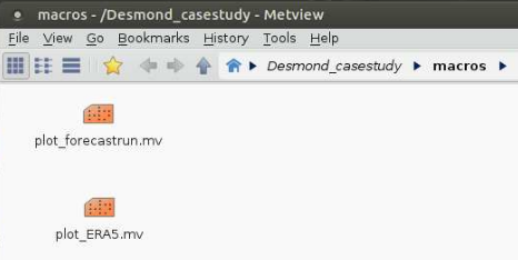 Image Added
Forecast maps
With right click on the macro and selecting Edit from the menu:
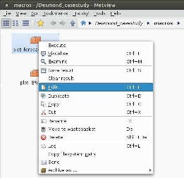 Image Added
a window pops up in which you can edit some parameters as meterorological variables to plot, geographical area, verification date:
 Image Added
After saving the modifications, the macro can be executed either from the macro window clicking on the blue arrow ( Image Added) in the top bar or with right click on the macro and selecting the Execute from the menu:
 Image Added
Figures can be saved selecting the Export menu point from the File menu. The timesteps are saved as individual pages in a multi-page .ps file.
 Image Added
Re-analysis maps
With right click on the macro and selecting Edit from the menu:
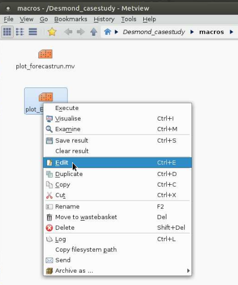 Image Added
a window pops up in which you can edit some parameters as meteorological variables to plot, geographical area, verification date. Please note that you can choose less variables here:
 Image Added
Figures can be saved in the same way as before. The timesteps are saved as individual pages in a multi-page .ps file.
| HTML |
|---|
At the end, you can compare your results (i.e. your plots) with the reference figures which are available on the <a href="http://download.ecmwf.int/test-data/openifs/reference_casestudies/oDesmond.html" target="_blank">ECMWF download server</a>.<a name="troubleshooting"></a> |
Troubleshooting
Here some cases are collected, when the model run and the forecast evaluation can terminate with error.
Model run
| HTML |
|---|
<ul>
<li class="li_withspace">The initial conditions are prepared for fix dates and spatial resolutions. Make sure that your settings coincide with that.</li>
<li class="li_withspace">The initial conditions are prepared with fix experiment ID that you can identify from the file names (e.g., in <span class="font_code_black">ICMGGgs0cINIT</span> experiment ID is <span class="font_code_black">gs0c</span>). Please make sure that you use the proper <span class="font_code_black">expID</span> in the job and the namelist, too.</li>
<li>Further possible issues regarding running the OpenIFS and their solution are listed in the <a href="https://confluence.ecmwf.int/display/OIFS/FAQ%3A+Frequently+Asked+Questions" target="_blank">OpenIFS FAQ</a>.</li>
</ul> |
Visualization with Metview
References
| HTML |
|---|
<p><a name="hersbach_2018"></a>Hersbach, H., de Rosnay, P., Bell, B., Schepers, D., Simmons, A., Soci, C., Abdalla, S., Alonso-Balmaseda, A., Balsamo, G., Bechtold, P., Berrisford, P., Bidlot, J-R., de Boisséson, E., Bonavita, M., Browne, P., Buizza, R., Dahlgren, P., Dee, D., Dragani, R., Diamantakis, M., Flemming, J., Forbes, R., Geer, A., Haiden, T., Hólm, E., Haimberger, L., Hogan, R., Horányi, A., Janisková, M., Laloyaux, P., Lopez, P., Muñoz-Sabater, J., Peubey, C., Radu, R., Richardson, D., Thépaut, J-N., Vitart, F., Yang, X., Zsótér, E., Zuo, H., 2018: <a href="https://www.ecmwf.int/sites/default/files/elibrary/2018/18765-operational-global-reanalysis-progress-future-directions-and-synergies-nwp.pdf" target="_blank">Operational global reanalysis: progress, future directions and synergies with NWP.</a> <em>ECMWF ERA Report Series 27</em>.</p>
<p><a name="hersbach_2016"></a>Hersbach, H., Dee, D.P., 2016: <a href="https://www.ecmwf.int/en/newsletter/147/news/era5-reanalysis-production" target="_blank">ERA5 reanalysis is in production.</a> <em>ECMWF Newsletter 147,</em> p. 7.</p>
<p><a name="szepszo_2018"></a>Szépszó, G., Carver, G., 2018: <a href="https://www.ecmwf.int/en/newsletter/156/news/new-forecast-evaluation-tool-openifs" target="_blank">New forecast evaluation tool for OpenIFS.</a> <em>ECMWF Newsletter 156,</em> 14–15.</p> |
Back to top
| CSS Stylesheet |
|---|
.cell_nopadding {
    padding: 3px;
    border: 0px;
}

.cell_leftmargin {
    padding-left: 30px;
}

.cell_top-bottom-border {
    border-top: 1px solid #3572b0;
    border-bottom: 1px solid #3572b0;
    border-left: 0px;
    border-right: 0px;
    padding: 3px;
}

.table_noborder {
     border: 0px;
}

.vertical {
    height: 100%;
}

.vertical td:first-child {
    position: relative;
    width: 35px;
    padding: 0;
    border: 2px solid #ddd;
}

.vertical_text {
    display: block;
    white-space: nowrap;
    -moz-transform: rotate(-90deg);
    -moz-transform-origin: center center;
    -webkit-transform: rotate(-90deg);
    -webkit-transform-origin: center center;
    -ms-transform: rotate(-90deg);
    -ms-transform-origin: center center;
    position: absolute;
    width:25px;
    color: #205081;
}

.table_line {
    padding: 0;
    height: 2px;
    border-left: 0px;
    border-right: 0px;
}

.table_line td:first-child {
    padding: 0;
    height: 2px;
    border-left: 0px;
    border-right: 0px;
}

.font_background_cyan {
    background-color: cyan;
}

.font_background_yellow {
    padding: 2px;
    background-color: #ffffb3;
}

.font_background_grey {
    padding: 2px;
    background-color: #dddddd;
}

.font_background_white {
    background-color: #ffffff;
}

.font_code_black {
    color: #000000;
    font-family: Monospace;
}

.li_withspace {
    margin-bottom: 10px;
}

.img_withoutspace {
    margin-bottom: -12px;
}

.font_background_darkgrey {
    padding: 2px;
    background-color: #aaaaaa;
}
|
| Excerpt Include |
|---|
| Credits |
|---|
| Credits |
|---|
| nopanel | true |
|---|
|

