In this tutorial we will demonstrate how how to run a forward simulation with FLEXPART and how to visualise the results in various ways.
...
| Code Block | ||
|---|---|---|
| ||
plot(view,g,conc_shade,title) |
Having run the macro we get a plot like this (after navigating to step 39h):
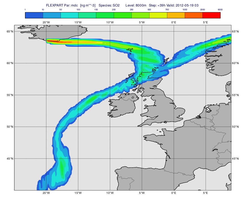
Computing and plotting total column mass
The macro to visualise the concentration fields on a given level is 'plot_total.mv'.
First, we define the level (8000 m) and the parameter ("mdc") we want to plot. Then we call mvl_flexpart_read_hl() to filter the data into a fieldset.
| Code Block |
|---|
dIn="result_fwd_conc/"
inFile=dIn  & "conc_s001.grib"
lev=8000
par="mdc"

#Read fields on the given height level
g=mvl_flexpart_read_hl(inFile,par,lev,-1,-1) |
Next, we define the contouring