...
| Expand | ||||||
|---|---|---|---|---|---|---|
| ||||||
|
...
This says that the release will happen over a 45 h period between heights 1651 and 10000 m at the location of the volcano and we will release 1000 tons of material in total.
| Info |
|---|
Please note that
|
The actual simulation is carried out by calling flexpart_run():
| Code Block | ||
|---|---|---|
| ||
#Run flexpart (asynchronous call!)

r = flexpart_run(
    output_path     	:   "result_fwd_conc",
    input_path      	:   "../data",
    starting_date   	:   20120517,
    starting_time   	:   12,
    ending_date     	:   20120519,
    ending_time     	:   12,
    output_field_type	:   "concentration",
    output_flux     	:   "on",
    output_trajectory   :   "on",
    output_area     	:   [40,-25,66,10],
    output_grid     	:   [0.25,0.25],
    output_levels   	:   [500,1000,2000,3000,4000,5000,7500,10000,15000],
    release_species 	:   8,
    receptors       	:   "on",
    receptor_names  	:   ["rec1","rec2"],
    receptor_latitudes  :   [60,56.9],
    receptor_longitudes :   [6.43,-3.5],
    releases        	:   rel_volcano
    )

print(r) |
Here we defined both the input and output path and specified the simulation period, the output grid and levels as well. We also told FLEXPART to generate gridded concentration fields and plume trajectories on output..
...
Next, we define the contouring definition. The units we used here is are ng m**-3 because for parameter "mdc" the native units (kg m**-3) are automatically scaled by the plotting library (see details about the this scaling for various FLEXPART GRIB fields here.
| Code Block | ||
|---|---|---|
| ||
#The contour levels
cont_list=[1,10,50,100,150,200,250,500,750,1000,2000,6000]

#Define contour shading
conc_shade = mcont(
    legend  						:   "on",
    contour 						:   "off",
    contour_level_selection_type    	:   "level_list",
    contour_level_list  			: 	cont_list,
    contour_label   				:   "off",
    contour_shade   				:   "on",
    contour_shade_method    		:   "area_fill",
    contour_shade_max_level_colour  :   "red",
    contour_shade_min_level_colour  :   "RGB(0.14,0.37,0.86)",
    contour_shade_colour_direction  :   "clockwise",
    contour_method: 					: 	"linear"
) |
Next, we build the title with mvl_flexpart_title(). Please note that we need to explicitly specify the plotting units!
...
| Code Block | ||||||
|---|---|---|---|---|---|---|
| ||||||
#Define coastlines coast_grey = mcoast( map_coastline_thickness : 2, map_coastline_land_shade : "on", map_coastline_land_shade_colour : "grey", map_coastline_sea_shade : "on", map_coastline_sea_shade_colour : "RGB(0.89,0.89,0.89)", map_boundaries : "on", map_boundaries_colour : "black", map_grid_latitude_increment : 5, map_grid_longitude_increment : 5 ) #Define geo view view = geoview( map_area_definition : "corners", area : [40,-25,66,9], coastlines : coast_grey ) |
and generate the plot:
| Code Block | ||
|---|---|---|
| ||
plot(view,g,conc_shade,title) |
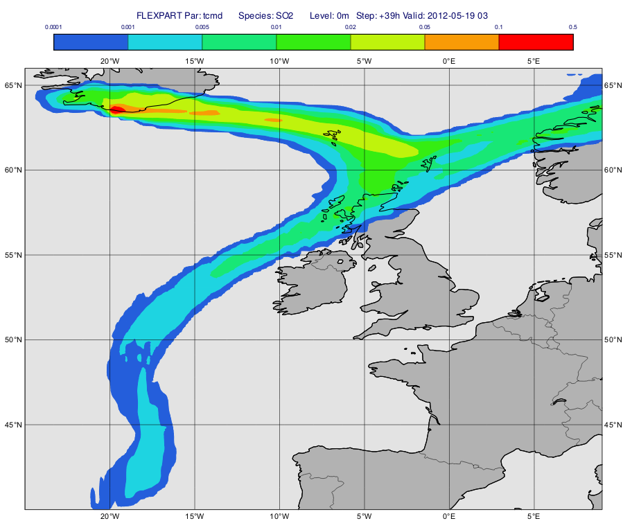
Having run the macro we will get a plot like this (after navigating to step 39h):
...
| Code Block | ||
|---|---|---|
| ||
title=mvl_flexpart_title(g,0.3,"g m**-2") |
Finally we define the view with the map in the same way as above
...
and generate the plot:
| Code Block | ||
|---|---|---|
| ||
plot(view,g,conc_shade,title) |
Having run the macro we will get a plot like this (after navigating to step 39h):
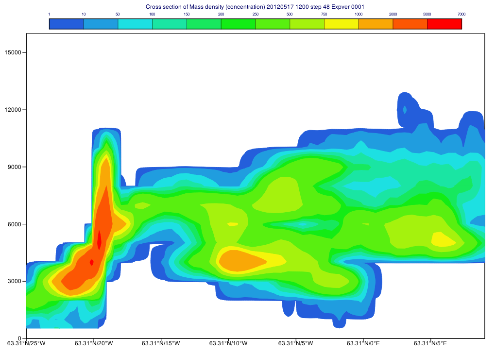
First, we define the parameter and time step for the cross section then call mvl_flexpart_read_hl() to extract the data. The result is a fieldset with units of "kg m**-3" that we need to explicitly convert to "ng m**-3" units for plotting since the automatic units scaling only works for map based plots.
| Code Block | ||
|---|---|---|
| ||
#Define level, parameter and step
lev=-1 #all levels
par="mdc"
step=48

#Get fields for all levels for a given step
g=mvl_flexpart_read_hl(inFile,par,lev,step,1)

#Scale into ng/m3 units
g=g*1000000000000
|
Next, we define the cross section view:
| Code Block | ||
|---|---|---|
| ||
xs_view = mxsectview(
	bottom_level	:	0,
	top_level	:	16000,
	line	:	[63.31,-25,63.31,9]
	)
|
Then, we define the contouring:
| Code Block | ||||||
|---|---|---|---|---|---|---|
| ||||||
#The contour levels
cont_list=[1,10,50,100,150,200,250,500,750,1000,2000,5000,7000]

#Define contour shading
conc_shade = mcont(
	legend	:	"on",
	contour	:	"off",
	contour_level_selection_type	:	"level_list",
	contour_level_list  : cont_list,
	contour_label	:	"off",
	contour_shade	:	"on",
	contour_shade_method	:	"area_fill",
	contour_shade_max_level_colour	:	"red",
	contour_shade_min_level_colour	:	"RGB(0.14,0.37,0.86)",
	contour_shade_colour_direction	:	"clockwise",
    contour_method: "linear"
) |
and finally generate the plot:
| Code Block | ||
|---|---|---|
| ||
plot(xs_view,g,conc_shade) |
Having run the macro we will get a plot like this: