For preparations and running the simulation needed for this tutorial click here ...
| Note |
|---|
To start these tutorial please enter folder 'forward'. |
Inspecting the FLEXPART GRIB file
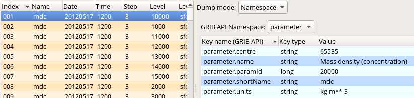
Before seeing the macro code to plot the data we inspect the file itself we work with. Double-click on the 'conc_s001.grib' GRIB icon' in folder 'result_fwd' to start up the Grib Examiner. We can see that our file contains the "mdc" (=Mass density concentration) fields we want to visualise. We can find out further details about this parameter by setting the Dump mode to Namespace and Namespace to Parameter in the examiner:
Generating the plot
The macro to visualise the concentration fields on a given level is 'plot_conc.mv'.
In the macro first we define the level (8000 m) and the parameter ("mdc") we want to plot. Then we call flexpart_filter() to extract the data.
| Code Block |
|---|
|
dIn="result_fwd/"
inFile=dIn  & "conc_s001.grib"
lev=8000
par="mdc"

#Read fields on the given height level
g=flexpart_filter(source: inFile,
                  param: par,
                  levType: "hl",
level: lev) |
Next, we define the contouring. The "mdc" fields have the units of "kg m**-3" but with the current value range "ng m**-3" units would better fit for contouring. To achieve this we simply multiply the "mdc" fieldset with 1012:
The contour definition itself goes like this:
| Code Block |
|---|
| language | py |
|---|
| title | Define contouring |
|---|
| collapse | true |
|---|
|
#The contour levels
cont_list=[1,10,50,100,150,200,250,500,750,1000,2000,6000]

#Define contour shading
conc_shade = mcont(
    legend  						:   "on",
    contour 						:   "off",
    contour_level_selection_type	:   "level_list",
    contour_level_list  			: 	cont_list,
    contour_label   				:   "off",
    contour_shade   				:   "on",
    contour_shade_method    		:   "area_fill",
    contour_shade_max_level_colour  :   "red",
    contour_shade_min_level_colour  :   "RGB(0.14,0.37,0.86)",
    contour_shade_colour_direction  :   "clockwise",
    contour_method					: 	"linear"
) |
Next, we build the title with flexpart_build_title(). Please note that we need to explicitly specify the plotting units!
| Code Block |
|---|
|
title=flexpart_build_title(data: g,fontsize: 0.3, units: "ng m**-3") |
Finally we define the map view:
| Code Block |
|---|
| language | py |
|---|
| title | Defining the map view |
|---|
| collapse | true |
|---|
|
#Define coastlines
coast_grey = mcoast(
	map_coastline_thickness			:	2,
	map_coastline_land_shade		:	"on",
	map_coastline_land_shade_colour	:	"grey",
	map_coastline_sea_shade			:	"on",
	map_coastline_sea_shade_colour	:	"RGB(0.89,0.89,0.89)",
	map_boundaries					:	"on",
	map_boundaries_colour			:	"black",
	map_grid_latitude_increment		:	5,
	map_grid_longitude_increment	:	5
	)

#Define geo view
view = geoview(
	map_area_definition	:	"corners",
	area				:	[40,-25,66,9],
	coastlines			: coast_grey
) |
and generate the plot:
| Code Block |
|---|
|
plot(view,g,conc_shade,title) |
Having run the macro we will get a plot like this (after navigating to step 39h):
