...
Please enter folder 'fwd' to start working.
Running the simulation
We will simulate a volcano eruption by releasing some SO2 from the Icelandic volcano Eyjafjallajökull.
...
| Info |
|---|
Please note that these are not the original outputs form FLEXTRA but were converted to formats more suitable for use in Metview. For details about the FLEXPART outputs please click here. |
Plotting concentration fields
To plot a particular parameter and level we need to filter the desired dataset from the resulting FLEXPART output file. Unfortunately, Metview's Grib Filter icon cannot handle these files (partly due to the local GRIB definition they use) so we need to use other means to cope with this task. For this reason and also to make FLEXPART output handling easier a set of Metview Macro Library Functions were developed. We will heavily use these functions in the examples below.
Inspecting the FLEXPART GRIB file
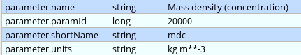
Before seeing the macro code to generate the plot we inspect the file itself we wanted to plot. Double-click on the 'conc_s001.grib' GRIB icon' in folder 'result_fw_conc' to start up the Grib Examiner. We can see that this file only contains "mdc" (=Mass density concentration) fields. We can find out further details about this parameter by setting the Dump mode to Namespace and Namespace to Parameter:
Generating the plot
The macro to visualise the concentration fields on a given level is 'plot_level.mv'.
...
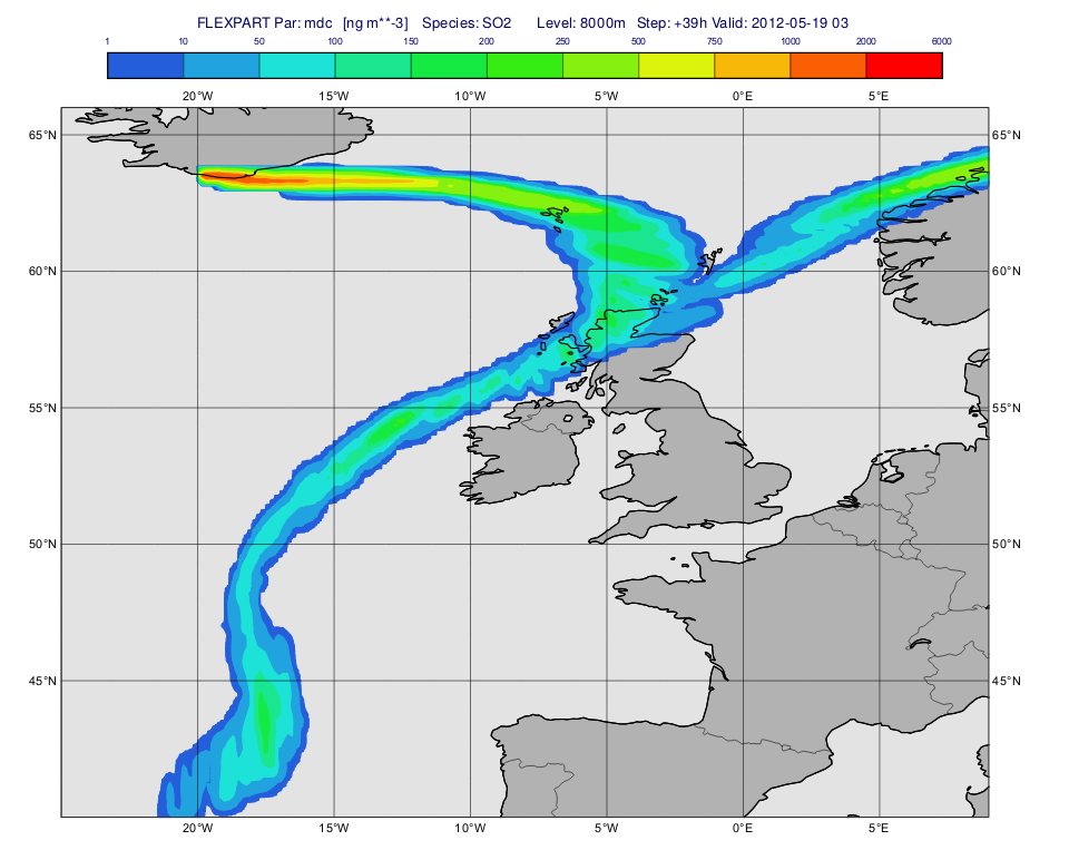
Having run the macro we will get a plot like this (after navigating to step 39h):
Plotting flux fields
To plot a particular parameter and level we need to filter the desired dataset from the resulting FLEXPART output file. Unfortunately, Metview's Grib Filter icon cannot handle these files (partly due to the local GRIB definition they use) so we need to use other means to cope with this task. For this reason and also to make FLEXPART output handling easier a set of Metview Macro Library Functions were developed. We will heavily use these functions in the examples below.
...
Next, we define the contouring definition. The units we used here are ng m**-3 because for parameter "mdc" the native units (kg m**-3) are automatically scaled by the plotting library (see details about the this scaling for various FLEXPART GRIB fields here.
Computing and plotting total column mass
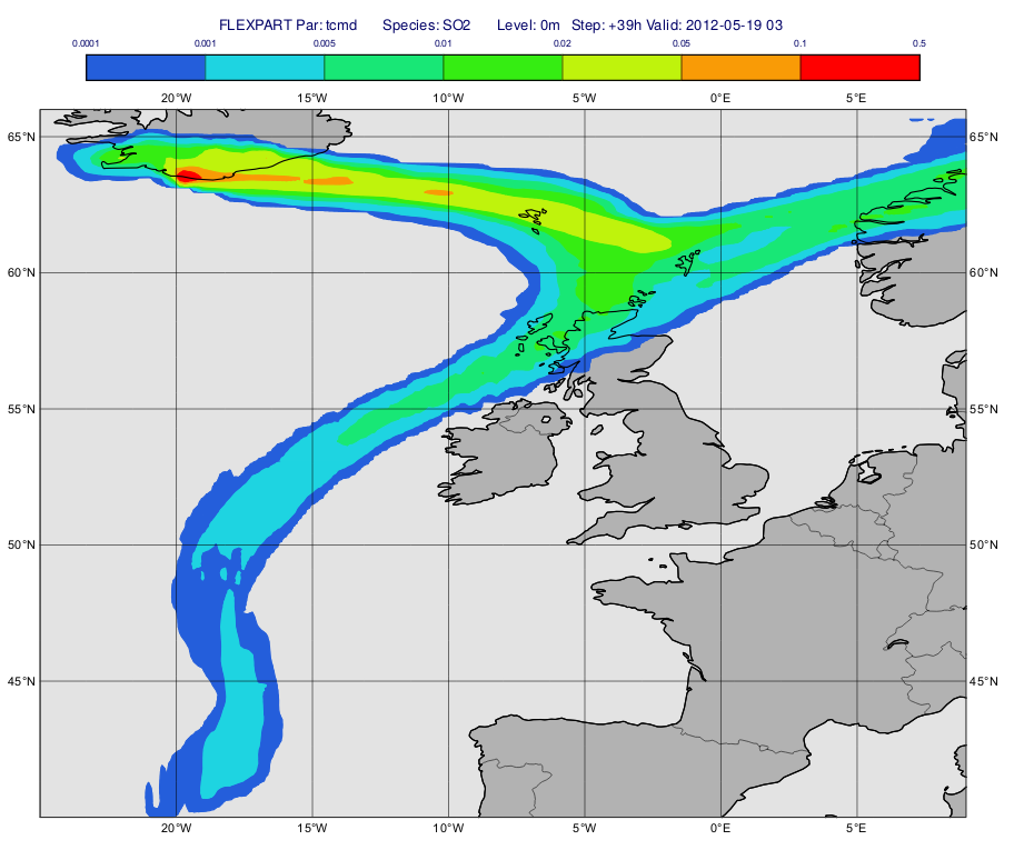
Using the same FLEXPART output as above we will compute and plot the total column integrated mass. The macro to use is 'plot_total.mv'.
...
Finally we define the view with the map in the same way as above and generate the plot:
| Code Block | ||
|---|---|---|
| ||
plot(view,g,conc_shade,title) |
Having run the macro we will get a plot like this (after navigating to step 39h):
...