Seasonal forecasts and the Copernicus Climate Change Service (C3S)
Introduction to seasonal forecasting
The production of seasonal forecasts, also known as seasonal climate forecasts, has undergone a huge transformation in the last few decades: from a purely academic and research exercise in the early '90s to the current situation where several meteorological forecast services, throughout the world, conduct routine operational seasonal forecasting activities. Such activities are devoted to providing estimates of statistics of weather on monthly and seasonal time scales, which places them somewhere between conventional weather forecasts and climate predictions.
In that sense, even though seasonal forecasts share some methods and tools with weather forecasting, they are part of a different paradigm which requires treating them in a different way. Instead of trying to answer to the question "how is the weather going to look like on a particular location in an specific day?", seasonal forecasts will tell us how likely it is that the coming season will be wetter, drier, warmer or colder than 'usual' for that time of year. This kind of long term predictions are feasible due to the behaviour of some of the Earth system components which evolve more slowly than the atmosphere (e.g. the ocean, the cryosphere) and in a predictable fashion, so their influence on the atmosphere can add a noticeable signal.
Seasonal forecasting within the C3S
The C3S seasonal forecast products are based on data from several state-of-the-art seasonal prediction systems. Multi-system combinations, as well as predictions from the individual participating systems, are available. The centres currently providing forecasts to C3S are ECMWF, The Met Office and Météo-France; in the coming months data produced by Deutscher Wetterdienst (DWD) and Centro Euro-Mediterraneo sui Cambiamenti Climatici (CMCC) will be included in the C3S multi-system.
Each model simulates the Earth system processes that influence weather patterns in slightly different ways, makes slightly different approximations, leading to different kinds of model error. These errors typically increase with the increase of integration time, so that the accumulated model errors become significant in comparison to the signal that the model is meant to predict. Some such errors are shared by the different models but others are not, so combining the output from a number of models enables a more realistic representation of the uncertainties due to model error. In most cases, such combined forecasts are, on average, more skilful than forecasts from the best of the individual models.
Currently, the C3S seasonal service offers graphical forecast products, available on the C3S web site, and public access to the forecast data, via the C3S Climate Data Store (CDS).
Seasonal forecasts are not weather forecasts: the role of the hindcasts
Seasonal forecasts are started from an observed state of (all components of) the climate system, which is then evolved in time over a period of a few months. Errors present at the start of the forecast (due to the imprecise measurement of the initial conditions and the approximations assumed in the formulation of the models) persist or, more often, grow through the model integration, reaching magnitudes comparable to that of the predictable signals. Some such errors are random; the effect of these on the outcome is quantified through the use of ensembles. Some errors, however, are systematic; if these systematic errors were determined, corrections could be applied to the forecasts to extract the useful information. This is achieved by comparing retrospective forecasts (reforecasts or hindcasts) with observations. The same forecast system is run for several starting points in the past in the same way as a forecast would be run (with only knowledge of the starting point), for the same length of time as an equivalent forecast. The resulting data set constitutes a 'climate' of the model, which can then be compared with the observed climate of the real world. The systematic differences between the model and the real world - usually referred to as biases - are thus quantified and used as the basis for corrections which can be applied to future, real-time forecasts. Given the relative magnitude of such biases, some basic corrections are essential to convert the data into forecast information - therefore a forecast by itself is not useful without relating it to the relevant hindcasts.
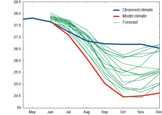
The image below is an example of the crucial role of the hindcasts in seasonal forecasting. It shows the time evolution of monthly-average temperature in a given region, between May and December: the blue line represents the average conditions observed over a period in the past (the reference period; in this case, 1993-2014), the red line is the equivalent model climate average over the same reference period. The difference between the two clearly indicates a significant cold bias, increasing with the time into the forecast. An ensemble of forecasts for a particular year is shown as green lines. When compared to the observed 'normal', all green ensemble predictions are for colder-than-normal conditions - not necessarily surprising when remembering that the model is systematically colder than the real world. However, when comparison is made with the model's 'normal' (the red line), all forecast ensemble members indicate warmer-than-normal conditions. Clearly, as the forecast is an output of the model, the latter comparison is the more appropriate.
As well as playing an essential role in the correction of systematic errors, hindcasts are also used to assess the skill of seasonal forecast systems (by comparing each of the forecasts for the years in the reference period with the respective observed conditions). Information on forecast skill is important to avoid overconfident decision making.
Note that for reasons related with the availability of computing resources, the hindcasts usually have fewer ensemble members per start date than the real-time forecasts, e.g. ECMWF SEAS5 5 has 51 members for the real-time forecasts, and just 25 members for the hindcasts.
Seasonal forecasting systems' versions and updates
Every forecasting system that contributes to C3S will have a different lifetime, so different versions of the systems are expected to be upgraded by their original institutions. For the real-time forecasts just one version of each one of the contributors will be made available to C3S at a given time. For instance, in November 2017 ECMWF changed its operational seasonal forecast system from system 4 to SEAS5, but both systems were kept running in parallel at ECMWF for a while. However, the only version of ECMWF seasonal forecasts available at C3S from November 2017 onwards is from SEAS5.
How do seasonal forecasting systems build their ensembles? And how are data produced?
"Burst" vs. "lagged" mode
In the last few decades, Earth system prediction has established the use of "ensemble" runs, to quantify the effect of errors due to both the uncertainty in the initial conditions and model deficiencies. This means that the forecasting systems produced a set of "slightly" different runs of the same forecast - the members of the ensemble - and thus the output of the forecast system is not a single solution, but a set of solutions. Since, by design, all ensemble members are equally likely, the forecast offers a distribution of outcomes, rather than a single deterministic answer.
Different techniques are used to build the members of an ensemble forecast, so that they sample the uncertainty in the initial conditions:
- "Burst" mode: all the members are initialized with conditions on the same start date, but from slightly different (perturbed) initial states, intended to sample the uncertainty in observations. (e.g. all members initialized on 1st March 2017; this is the case for ECMWF's system)
- "Lagged" mode: members are initialized on different start dates, the differences between which are sufficiently small (e.g. members initialized every day of the month; this is the case for Met Office system)
Among the systems that contribute to the C3S seasonal forecasts, some use "burst" mode, others lag the start dates of the members of their ensembles. For more details, refer to the table below in the "Production schedules" subsection.
Fixed vs. on-the-fly hindcasts
For several reasons, from computer load balance to flexibility in the introduction of changes in the systems, the different seasonal forecast contributors to C3S use different schedules to produce their hindcast sets:
- fixed hindcasts. Some systems are designed so their expected lifetime will be around 4-5 years. Once the system has been designed and tested, ensemble hindcasts for the whole reference period are run. The advantage is that this reference dataset is available well in advance of real-time forecasts being issued, and its properties (biases, skill) can be quantified once for repeated use. As this is a very expensive exercise, it cannot be repeated too often and thus the system remains fixed for a long period of time.
- on-the-fly hindcasts. Some systems prioritise more frequent upgrades, which means that the hindcast sets have to be run more frequently. To achieve this in practice, the full hindcast set is run every time a new real-time forecast is produced, slightly in advance (a few weeks) of the real-time forecast and using exactly the same version of the forecasting system. This also offers the advantage of balancing the requirement for computing resources, but the compromise is the regular change of the model climatology.
Production schedules for the seasonal forecasting systems contributing to C3S
The following summarises the information about the ensemble sizes, start dates and production schedule for the seasonal forecasting systems contributing to C3S.
| SYSTEM | FORECASTS | HINDCASTS | |||
|---|---|---|---|---|---|
| ENSEMBLE SIZE and START DATES | PRODUCTION | ENSEMBLE SIZE and START DATES | PRODUCTION | ||
| ECMWF | System 4 (CDS system: 4) | 51 members start on the 1st | real-time | 15 members start on the 1st | fixed dataset |
SEAS5 | 51 members start on the 1st | real-time | 25 members start on the 1st | fixed dataset | |
| Météo-France | System 5 | 51 members (a) 26 start on the first Wednesday after the 19th | real-time | 15 members start on the first Wednesday after the 19th (a) | fixed dataset |
| System 6 (CDS system: 6) | 51 members 1 starts on the 1st | real-time | 25 members 1 starts on the 1st | fixed dataset | |
System 7 | 51 members 1 starts on the 1st | real-time | 25 members 1 starts on the 1st | fixed dataset | |
| Met Office | GloSea5 (b) (CDS system: 12,13, 14, 15 (d)) | 2 members start each day (c) | real-time | 7 members on the 1st | on-the-fly produced around 4-6 weeks in advance |
| CMCC | SPSv3 | 50 members start on the 1st | real-time | 40 members start on the 1st | fixed dataset |
| DWD | GCFS2.0 (CDS system: 2) | 50 members start on the 1st | real-time | 30 members start on the 1st | fixed dataset |
| NCEP | CFSv2(b) | 4 members start each day 1 member per start hour: 0, 6, 12, 18 | real-time | 4 members start every 5 days (e) 1 member per start hour: 0, 6, 12, 18 | fixed dataset |
(a) Despite being produced in a lagged mode, the data from Météo-France forecasting systems is currently encoded and provided in CDS as if all the members were initialized on the 1st.
(b) The production schedules of forecasting system with lagged start dates don't prescribe how to build an ensemble for a specific nominal start date. The choices currently in use for the C3S products for those forecasting systems can be found within the information about the concept of nominal start date.
(c) Due to the flexibility of the Met Office forecasting system, forecast failures on a given date are not usually recovered by re-running the missed forecasts at a later date, but by running more members with initial conditions of the day of recovery.
Example: An incident affected the 22 August 2017 forecast so no members are available for that date. Instead, 4 members were initialised on 23 August 2017.
(d) For the Met Office contribution, due to the production of hindcasts "on-the-fly", the CDS keyword 'system' does not have the same meaning as for the other contributors. Instead, it is just an indexing label that gets changed once per year.
(e) Details of the complete list of start dates are provided in the description of CFSv2 system, section 6. Other relevant information