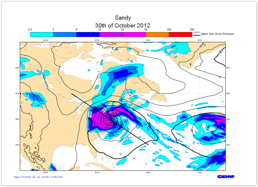
You are viewing an old version of this page. View the current version.

Compare with Current View Page History

« Previous Version 11 Next »


Objectives


  • Set-up a cylindrical projection over the United States.
  • Apply land-sahding on the coastlines.
  • Load a grib file containing Mean-Sea level Presssure and visualise it using black isolines.
  • Load a grib file containing Precipitation  and visualise it using shading technique.
  • Add a legend.
  • Add a text.
  • Draw the position of New-York City
  • Draw a line to materialise the Xsection we are going to visualise in a next tutorial

You will need to download


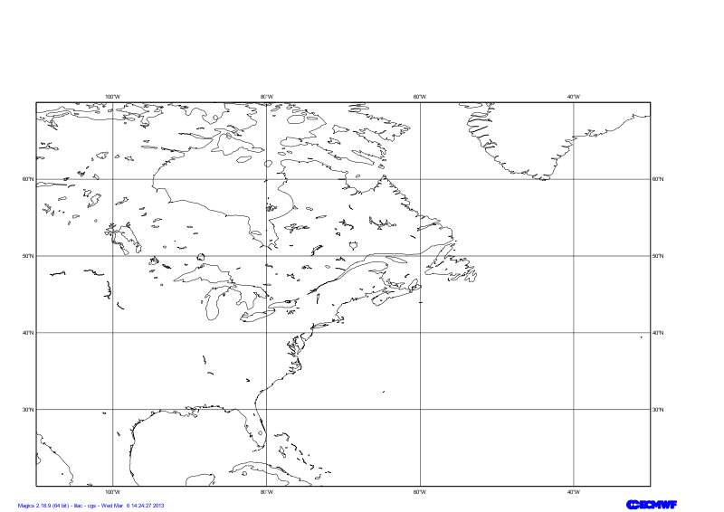
Setting of the geographical area

The Geographical area we want to work with today is defined by its lower-left corner [20oN, 110oE] and its upper-right corner [70oN, 30oE].

Have a look at the  subpage documentation to learn how to setup a projection .

Parameters to check


subpage_lower_left_longitude

subpage_lower_left_latitude
subpage_upper_right_longitude
subpage_upper_right_latitude
Python - Setting a projection
from Magics.macro import *
#setting the output 
output = output(    
                output_formats = ['png'],
                output_name = "map_step1",
                output_name_first_page_number = "off"
        )
#settings of the geographical area 
area = mmap(subpage_map_projection="cylindrical",
        subpage_lower_left_longitude=-110.,
        subpage_lower_left_latitude=20.,
        subpage_upper_right_longitude=-30.,
        subpage_upper_right_latitude=70.,
    )    
#Using a default coastlines to see the result
plot(output, area, mcoast())


Setting the output

The object output allows the definition of the output format, and the settings of the output file name .

Have a look at the  PNG output documentation  to see which parameters are available to set-up a PNG output.

To create a PNG output Magics, you have to create an output object and to insert at the first position in the plot command


Python - Output
from Magics.macro import *

#settings of the png output 
output = output(
			output_formats = ['png'],
  			output_name = "magics",
    		output_name_first_page_number = "off"
    )

#The plot commad will create a png output called magics.png
plot(output, mcoast())

Setting the coastlines

The object mcoast allows the parametrisation of the coastlines.

To configure the look of your coastlines you have to create a mcoast object with the parameters you want.

The mcoast object has to be inserted in the plot command.

Python - Coastlines
from Magics.macro import *

#settings of the png output 
output = output(
			output_formats = ['png'],
  			output_name = "coast",
    		output_name_first_page_number = "off"
    )
##settings of the coastlines attributes 
coast = mcoast(
  map_coastline_land_shade = "on",
  map_coastline_land_shade_colour = "cream",
  map_grid_line_style = "dash",
  map_grid_colour = "brown",
  map_label_colour = "brown",
  map_coastline_colour = "brown"
)

#The plot command will now use the coast object
plot(output, coast)


Adding a text

Magics allows the user to add of or several lines of text. The position of the text is by default above the plot, but some parameters aloow it to be moved around.

A basic html formatting can be used for colour, style, and font size.

The mtext object has to be inserted in the plot command to see the text on the result.


Python - Title
from Magics.macro import *

#settings of the png output 
output = output(
			output_formats = ['png'],
  			output_name = "coast",
    		output_name_first_page_number = "off"
    )
##settings of the coastlines attributes 
coast = mcoast(
  map_coastline_land_shade = "on",
  map_coastline_land_shade_colour = "cream",
  map_grid_line_style = "dash",
  map_grid_colour = "brown",
  map_label_colour = "brown",
  map_coastline_colour = "brown"
)
##settings of the text (notice the Html formatting)
title = mtext(
  text_lines = ["Hello World!", " <b>This is my first plot</b> !"],
  text_font_size = "0.7",
  text_colour = "charcoal"
  )
#The plot command will now use the coast and title objects
plot(output, coast, title)


  • No labels