Introduction
One of Metview's most powerful features is its data processing ability. Data from various sources can be combined and manipulated using high- or low-level commands.
XXXX Download data
Fieldset Manipulation
A fieldset is a collection of fields stored physically in GRIB files. Metview has many built-in functions and operators to manipulate fieldsets, from simple arithmetic operators to vertical integrations through the atmosphere. Many of these operations are available from the icon-based user interface, all are available in the Macro language. The results can be stored on disk, or passed to other functions for further manipulation.
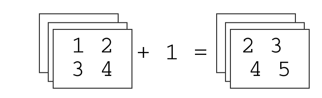
Most of these functions work on each gridpoint value of each field in the fieldset. For example, if we add 1 to a fieldset which contains 3 fields, this will return a new fieldset with 3 fields, the values of which are 1 greater than their respective input fields, as shown below:
The situation is similar for operations between two fieldsets:
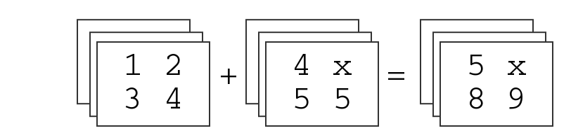
This example also illustrates what happens when missing values are in the data, represented here by an "x". In most cases it is not valid to use the missing value in the result, so that point in the result will itself be set to the missing value indicator.
Computing a Forecast - Analysis Difference

As a simple example, let's compute the difference between a set of forecast fields and the corresponding set of analysis fields for the same time step.
Have a look at the supplied GRIB files (right-click, examine) to confirm that temperature_forecast.grib contains, at multiple vertical levels, 48-hour temperature forecasts for the same date and time as the analysis data in temperature_analysis.grib.
Create a new Simple Formula icon and rename it to fc_an_diff. Edit the icon, ensure that the first tab is selected (F+G) and that the operator is minus ( - ). Drop your temperature_forecast.grib icon into the Parameter 1 box, and drop temperature_analysis.grib into the Parameter 2 box. Save the icon and execute it. The icon should turn green, indicating the result has been computed and cached. Further operations on this icon will not re-compute the result unless either of its input icons are modified. If you simply wanted the result to be stored, you could right-click and choose save result to bring up a file save dialogue; but instead choose visualise to plot it. Note that all 6 fields in each data icon are used in the computation - the result is a set of 6 fields.
The solutions folder contains two Contouring icons which can be used to show the differences. Drop pos_shade and then neg_shade into the Display Window. Notice that the second one replaces the first one - this is not what we want! Select both icons with the mouse and drop them both together into the Display Window to use them both in the plot. Edit the icons to see which parameters were used to create the positive and negative shading effects. There is also a Contouring icon called rainbow_diffs - this uses Metview's ability to draw isolines of different colours rather than using shading. This can be useful if it is important to see another layer underneath the temperature.
We could have done this a bit quicker - there was no need to execute the fc_an_diff icon. If you right-click the icon and choose clear result, you can now directly choose visualise - the execute action is performed in the background, as it is required before visualisation can occur.
Putting it into a Macro
Ensure that the difference fieldset is visualised with the contouring applied. One way to generate a Metview Macro script from this plot is to click the Generate Macro button (also available from the File menu). A new Macro script will be generated - have a look at it to confirm that it contains code to read the data, compute the difference and plot the result. Run the macro to obtain the plot, either by using the Run button from the Macro Editor, or by selecting visualise from the icon's context menu). By default, the macro is written so that it will produce an interactive plot window; it will generate a PostScript file if it is run with the execute command, or if it is run from the command line.
Notice how simple the computation of the field differences is:
fc_an_diff = temperature_forecast - temperature_analysis
The variables temperature_forecast and temperature_analysis are fieldset variables, coming, as they do, from GRIB data. Any operation on or between fieldsets is applied to every grid point in every field in the fieldset. Metview Macro has a large set of functions and operators on fieldsets.
Computing a Forecast - Observation Difference
This time we'll compare two very different data types: gridded forecast data in a GRIB file, with scattered observation data described in a BUFR file. We will use the t2m_forecast icon (the gridded forecast data), and the observation data is in a BUFR file represented by the obs.bufr icon and contains observations over Europe, valid at the same time as the GRIB data. Examine and visualise both icons to confirm what they contain.
Extracting the 2 metre temperature
The first step to comparing GRIB data with BUFR data is to extract just the parameter we want from the BUFR data and convert it to the geopoints format. Then the computation will be simple.
Create a new Observation Filter icon and rename it to filter_obs_t2m.
| Data | Drop the obs.bufr icon here |
| Output | Geographical Points |
| Parameter | 012004 |
Note that 012004 is the code for 'Dry bulb temperature at 2m'. Confirm that the result of this icon's filtering is a set of geopoints with temperature values.
Computing the forecast-observation difference
This is just the same as before, using a Simple Formula icon; create a new one and rename it to fc_obs_diff. Drop t2m_forecast into the Parameter 1 box, and filter_obs_t2m into the Parameter 2 box. Notice how we are chaining together a sequence of icons - the output of the Observation Filter icon is an input to the Simple Formula icon. Any number of icons can be chained together like this.
Visualise the result - you will see that the result of a field minus a scattered geopoints data set is another geopoints data set. For each geopoint location, the interpolated value from the field was extracted before performing the computation. From the solutions folder, drop both the diff_symb_hot and the diff_symb_cold icons together into the plot in order to get a more graphical representation of the result.
XXXXX
Putting it into a Macro
As with the previous exercise, create a macro which will run all of these steps and plot the result. We could do it using the Generate Macro button from the Display Window, but this time we will do it another way. Create a new Macro icon, rename it to plot_fc_obs_diffs and edit it. Drop the fc_obs_diff icon into the Macro editor - the whole chain of icons which act as input to this one are included in the generated code. Drop also diff_symb_hot and diff_symb_cold into the editor and add a plot() command:
plot(fc_obs_diff, diff_symb_hot, diff_symb_cold)
Computing Wind Speed from U/V
The GRIB file uv850 contains analysis data for U and V wind components at 850hPa. The task is to compute the wind speed from this using a macro, so create a new Macro icon, rename it compute_wind_speed and edit it.
Perform the following steps:
- filter the U wind component into a variable called
u(you may find it useful to use the GRIB Filter icon to do this and then drop it into the Macro Editor) - filter the U wind component into a variable called
v apply the formula
speed = sqrt(u*u + v*v)- plot the result
Returning a Computation for Further Interactive Use
The result of the above macro does not have to live entirely inside the macro - it can be passed back to the user interface or used as input to other icons. Do this:
- in the above macro, comment out the
plot()command (using the hash,#, symbol) - add a new line of code at the end:
return speed
This passes the fieldset speed back to the user interface. Try it by right-clicking on the macro's icon and selecting examine, save or visualise.
Field Interpolation
Metview's GRIB Filter icon has parameters which enable the interpolation of data onto a new grid, or the extraction of a sub-area. This can be useful if you wish to compare two fields which are currently at different resolutions (e.g. from different model runs) - both fields need to be on the same grid before Metview can perform computations between them.
The GRIB icon reduced_gg_320 contains one field which is stored as a reduced Gaussian grid. Visualise the field and apply the gridpoints icon (in the solutions folder) to display the locations of the grid points.
Now create a new GRIB Filter icon with these parameters:
| Data | Drop the reduced_gg_320 icon here |
| Grid | 2/2 |
The result will be the same data interpolated onto a 2x2 degree grid. Visualise the result and apply the gridpoints icon to confirm the new grid. Visualise the two fields side-by-side with coloured contour shading to also confirm that they look very similar in terms of their data values.
Conversion Between Points and Fields
Metview provides two icons, Geopoints to GRIB and GRIB to Geopoints for the purpose of converting between GRIB (gridded) and geopoints (scattered) formats.
Use a GRIB to Geopoints icon to convert the result of the last exercise to geopoints format. Examine the result to confirm that it is now geopoints and that we have a list of all the individual points.
Use a Geopoints to GRIB icon to convert the geopoints result of the fc_obs_diff icon to GRIB.
Extra Tasks
Computing relative differences
Adapt the macros from this tutorial so that they compute relative differences rather than absolute differences between the values. By this we mean compute the differences as percentages of the original analysis values. You will need to create new Contouring and Symbol Plotting icons to plot these nicely.
Overlaying wind speed with wind arrows
Write a macro which takes U and V wind components from a GRIB file and plots the wind speed as shaded contours with wind arrows overlaid on top.