Overview

Time is a very important dimension in meteorology, and there are many things to keep in mind. Here we will explore how Metview handles the fourth dimension.

XXX download

Overlaying Time Steps

Inspect the supplied GRIB files: z500_fc.grib contains geopotential forecasts made in one run, but for six different forecast steps; z500_an.grib contains analysis fields for two times. Visualise the supplied Geographical View icon and drop the forecast GRIB icon along with its corresponding Contouring icon into the Display Window, and then drop the analysis GRIB icon along with its corresponding Contouring icon too. Go through the frames of animation. The fields have been overlaid, but if you look at the times and dates in the title, you will see that they do not match. Metview has simply plotted the first field of each data file together, then the second, and so on. We can make it more intelligent.

Edit the Geographical View icon and set this:

Save the icon, visualise it and drop the data with their visdefs in again. Go through the animation steps and look at the Frames tab in the Display Window to see what has happened. Now the fields will be overlaid only if their valid date and time match.

Metview's overlay rules

To summarise, Metview's overlay rules can be described like this:

In practice, this means that a GRIB file with 5 fields is visualised as 5 separate plots which you can scroll through.

If you wish to overlay data, then you must provide separate data icons for each 'layer'. Then we are subject to Rule 2:

Hovmoeller?

Precipitation

Precipitation data provides an interesting challenge. Precipitation fields in MARS are stored as accumulated fields. Visualise the supplied precip.grib icon with the precip_shade visdef. The first field is empty (check using the Cursor Data). The first field has a step of 0, meaning that it contains the total precipitation accumulated between the run time and the run time plus step. Since these are the same, there is no accumulated precipitation! Subsequent steps show more and more precipitation (the amount accumulated over 3, 6, 9, etc hours).

What if we want to plot just the rain that accumulated between 06:00 and 09:00? That would be the accumulated precip at 09:00 minus the accumulated precip at 06:00. We can compute this in a macro.

Create a new Macro icon and rename it compute_precip.

We can see from examining the file that the 6 and 9 o-clock steps are fields 3 and 4 respectively (using 1-based indexing). So the following macro code will compute the difference and return it:

precip = read("precip.grib")

precip_6_to_9 = precip[4] - precip[3]
return precip_6_to_9

Visualise the macro to plot it.

Now we want to go further and compute the precipitation for each and every 3-hour period. We can do this with more complex field indexing.

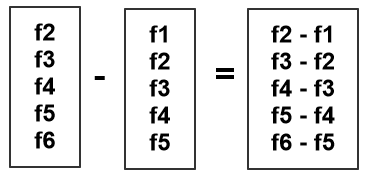
So we want field 2 minus field 1, field 3 minus field 2, etc. We can do this in a single line of code because we can handle multiple fields in a single operation as shown:

To extract fields 1 to 4, for example, we can use the following syntax:

fields = precip[1,4]

So the following piece of code will do what we want in a more general way:

precip = read("precip.grib")

n = count(precip) # the number of fields in the fieldset
precip_3h = precip[2, n] - precip[1, n-1]
return precip_3h

Visualise the macro. Your plot may be blank! There is one more trick: we have created a derived field, and this changes the automatic scaling algorithm used when plotting. Precipitation is stored in metres, but we want to display it in mm. Modify the precip_shade icon and set:

Visualise your macro result again and confirm that you now have precipitation only for the 3-hour periods, which does not accumulate with each frame.

Note that the meta-data for each field is taken from the first field in each subtraction; "step9 minus step6" returns a field with meta-data from step9, so be aware of this. Macro has functions for setting GRIB meta-data if you need to change it in order to correctly describe the new data.

Dates in Macro

Macro has specific date-handling abilities. Dates are a built-in data type which in fact describe both a date and a time.

Defining dates

You can create date variables in a number of ways:

• yyyy-mm-dd
• yyyy-DDD  (DDD is a 3-digit Julian day, e.g. 365 is 31st December in non-leap years)

These will have the time set to 00:00. A different time can be added by adding

• HH:MM
• HH:MM:SS

Create a new Macro icon, rename it to dates and define a date:

d1 = 2015-03-11
print(type(d1))
print(d1)

Try adding a time:

d1 = 2015-03-11 12:00

Converting numbers into dates

The date() function converts numbers into dates using the same syntax that MARS understands. For example:

• d1 = date(20150105)
• today = date(0)
• yesterday = date(-1)

This syntax can be useful if reading dates from a text file or some other source.

Again, the time will be 00:00 unless we add it. We can consider the time to be a fraction of a day:

• midday = date(20150105.5)

Use this syntax to add another variable, d2, which contains the date and time for 13:00h at 2015-03-13. Print it to check it.

Note that when passing numeric dates such as 20150105 to other modules, such as the MARS Retrieval module, these do not need to be converted into date variables.

Date arithmetic

When dealing with dates, the number 1 represents one day. So the expression d1 + 1 gives a date one day later than day 1. To compute the difference, in days, between two dates, it's simply:

• diff = d2 - d1

Times can be added as fractions of days, and there are some helper functions too:

• d1 = d1 + 0.5                               # add 12 hours
• d1 = d1 + hour(12)                          # hour(12) returns 0.5
• d1 = d1 + hour(23) + minute(58) + second(0) # 2 minutes to midnight

Compute and print the difference between your two dates, d2 and d1.

Looping through dates

Three examples, to get a feel for it:

for d = 2015-01-01 to 2015-03-01 do
    print(d)
     ... # each step is 1 day
end for

for d = 2015-01-01 to 2015-03-01 by 2 do
    print(d)
     ... # each step is 2 days
end for

for d = 2015-01-01 to 2015-03-01 by hour(6) do
    print(d)
    ... # each step is 6 hours
end for