Introduction
Metview has much functionality for meteorological data types stored in ECMWF's MARS archive, for example GRIB, BUFR and ODB. But not all data comes in these formats. Therefore Metview has facilities to handle various other data types, which we will explore here.
Visualiser Icons
Some formats, such as GRIB, are easy to visualise in Metview - just right-click, Visualise. This is because they are quite constrained in their contents and have enough standardised meta-data for a program to understand how they should be plotted. Some other formats, such as netCDF and tables of ASCII data are not easily interpreted for automatic plotting (which variables/columns should be selected and what do they represent?). Metview introduces the concept of the Visualiser icon, which we will use in some of the following examples.
NetCDF
NetCDF is a binary file format for storing multi-dimensional arrays of data and enjoys wide academic usage.
Examining netCDF

Right-click on the supplied netcdf.nc icon and choose examine to see its structure. It consists of multi-dimensional variables, each of which has its own set of attributes; the file also has a set of global attributes.
Visualising netCDF
Create a new NetCDF Visualiser icon. Edit it and drop the netcdf.nc icon into the NetCDF Data field. Set the following parameters:
| Netcdf Plot Type | Geo Matrix |
| Netcdf Latitude Variable | latitude |
| Netcdf Longitude Variable | longitude |
| Netcdf Value Variable | v2d |
Save the changes, and visualise this new icon. See how the settings in the visualiser icon correspond to the variable names in the data. Now visualise another field from the same file. Use the supplied shading_20_levels icon on the plots.
Geopoints
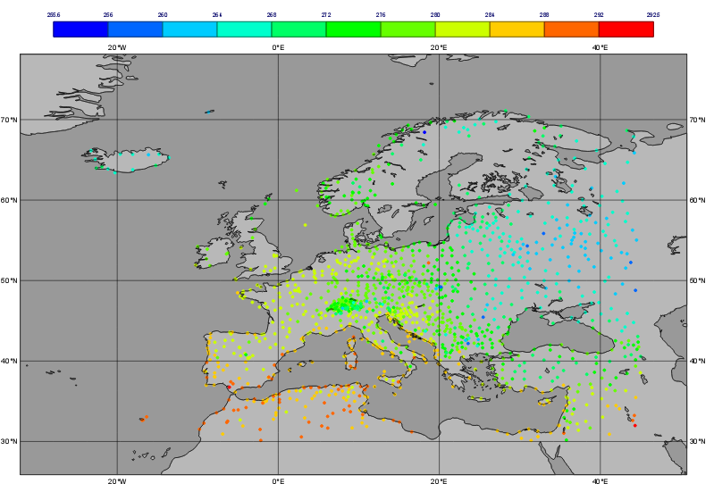
Format overview
Geopoints is the ASCII format used by Metview to handle spatially irregular data (e.g. observations). There are a number of variations on the format, but the default one is a 6-column layout. The columns do not have to be aligned, but there must be at least one whitespace character between each entry.
This example shows a geopoints file containing dry bulb temperature at 2m (PARAMETER = 12004).
#GEOPARAMETER = 12004lat long level date time value#DATA36.15 -5.35 0 19970810 1200 300.934.58 32.98 0 19970810 1200 301.641.97 21.65 0 19970810 1200 299.445.03 7.73 0 19970810 1200 29445.67 9.7 0 19970810 1200 302.244.43 9.93 0 19970810 1200 293.4 |
If you have observation data which you wish to import into Metview, Geopoints is probably the best format because:
- it is easy to write data into this format
- Metview has lots of functions to manipulate data in this format
Variants of the format allow 2-dimensional variables to be stored (e.g. U/V or speed/direction wind components), and another variant stores only lat, lon and value for a more compact file.
Examining geopoints
Examine the supplied geopoints.gpt icon to confirm the contents of the file. The columns are sortable. You may wish to open the file in an external text editor to see exactly what it looks like.
Visualising geopoints
Visualise the icon. The visdef used for geopoints is Symbol Plotting, and its default behaviour is to plot the actual numbers on the map. This can become cluttered, and text rendering can be slow. Drop the supplied symb_colours icon into the Display Window to get a better view of the data (you can also edit symb_colours to see which parameters were set to achieve this effect.
Computing some statistics in Macro
First, we will print some information about our geopoints data. Create a new Macro icon, type this code and run it:
gp = read('geopoints.gpt')
print('Num points: ', count(gp))
print('Min value: ', minvalue(gp))
print('Max value: ', maxvalue(gp))
Perform a simple data manipulation and return the result to Metview's user interface:
return gp*100
Save the macro and see its result by right-clicking on its icon and choosing examine or visualise. We could also have put a write() command into the macro to write the result to a geopoints file.
Finding geopoints points within 100km of a given location
As a more complex example, we will combine two functions in order to find the locations of the points within a certain distance of a given location. We will use the same geopoints file as before.
The distance() function returns a new geopoints variable based on its input geopoints, where each point's value has been replaced by the distance of that point from the given location. The description of this function follows:
geopoints distance ( geopoints,number,number )
geopoints distance ( geopoints,list )
Returns geopoints with the value of each point being the distance in metres from the given geographical location. The location may be specified by supplying either two numbers (latitude and longitude respectively) or a 2-element list containing latitude and longitude in that order. The location should be specified in degrees.
Choose a location and use this function to compute the distances of the data points from it. Assign the result to a variable called distances and return it to the user interface to examine the numbers. The distances are in metres.
Now we will see a boolean operator in action. The expression distances < 100000 (one hundred thousand) will return a new geopoints variable where, for each point, if the input value was less than 100000, the resulting value will be 1; otherwise the resulting value will be zero. So the resulting geopoints will have a collection of ones and zeros. Confirm that this is the case.
The filter() function, from the documentation:
geopoints filter ( geopoints,geopoints )
A filter function to extract a subset of its geopoints input using a second geopoints as criteria. The two input geopoints must have the same number of values. The resulting output geopoints contains the values of the first geopoints where the value of the second geopoints is non-zero. It is usefully employed in conjunction with the comparison operators :
freeze = filter(temperature,temperature < 273.15)
The variable freeze will contain a subset of temperature where the value is below 273.15.
Use this in combination with what you have already done to produce a geopoints variable consisting only of the points within 100km of your chosen location. Plot the result to confirm it.
Saving geopoints data
Geopoints variables can be saved to disk using the write() command:
write('my_computed_data.gpt', points)
Converting between geopoints and GRIB
This has already been covered in Data Part 1.
Other ASCII Data
ASCII Table Data
Metview incorporates functionality to read, process and visualise data stored in ASCII table files, including the commonly-used CSV (comma-separated value) format.
Visualising ASCII table data
Look at the supplied file t2_20120304_1400_1200.csv. This is a standard CSV file, with a header row at the top, followed by one row per observation, one column per field.
Station,Lat,Lon,T2m
1,71.1,28.23,271.3
2,70.93,-8.67,274.7
. . .
A CSV file can have any number of columns, but this is a simple example.
To plot the data, we need to tell Metview which columns contain the coordinates and which contain the values. Create a new Table Visualiser icon and edit it. Drop the CSV icon into the Table Data field and set the following parameters:
| Table Plot Type | Geo Points |
| Table Longitude Variable | Lon |
| Table Latitude Variable | Lat |
| Table Value Variable | T2m |
Notice that this icon contains several parameters at the bottom which allow you to read differently-formatted ASCII table files. The question-mark buttons beside the parameter names give brief information on what they mean. The defaults are set up to read a standard CSV file, so we don't need to touch these parameters in this example.
Visualise this icon to plot the data, and apply the supplied symb_colours icon to get a nicer plot.
Converting ASCII Table data to geopoints format
Although Metview has some functionality for handling this type of data in Macro, it can do much more with the geopoints format. Therefore, if the data points are in geographic coordinates, one useful exercise is to read one of these files and convert it to geopoints.
Create a new Table Reader icon - this is purely a helper icon which exists only to aid the generation of Macro code. Drop the CSV file into the Data field. We do not need to touch the other parameters since this is a standard CSV file.
Drop the icon into a new Macro to generate the code to read the file. Rename the resulting variable to data. The following lines of code will print some information about the data:
print('Num cols: ', count(data))
print('Col 4: ', name(data, 4))
Now we will create a new geopoints variable, and set its lats, lons and values to those from the CSV data.
First, use the values() function to extract arrays of lats, lons and T2m from the CSV data. These will be returned in variables of type vector - this is an in-memory array of double-precision numbers.
vector or list values( table, number )
vector or list values( table, string )
Returns the given column specified either by an index (starting at 1) or a name (only valid if the table has a header row). If the column type is number, a vector is returned; if it is string, then a list of strings is returned. If the column cannot be found, an error message is generated.
Next, find out how many values there are, using the count() function on one of the returned vectors.
Finally, the following code shows how to construct a simple geopoints variable using only these columns (i.e. it will be in XYV format):
geo = create_geo(num_vals, 'xyv')
geo = set_latitudes (geo, lats)
geo = set_longitudes(geo, lons)
geo = set_values    (geo, vals)
The macro can now write this to disk, return it to the user interface or process it further using all the available geopoints functions.
ASCII Lat / Lon Matrices
Have a look at the supplied Lat Lon Matrix file with the edit action. This is a simple text format for storing regularly-spaced geographical matrix data, which Metview can directly import. As soon as you do anything with this file (e.g. visualise or examine), Metview internally converts it into GRIB format (leaving the original file untouched). In this way, we can import such data into Metview and have access to all its GRIB/fieldset functionality.
Reading/Writing General ASCII Data to/from Disk
ASCII files that are not in Geopoints, ASCII Table or Lat/Long Matrix format can be read using the read() function. It will return a list of strings - one string will contain the contents of one line of the file. Look at the supplied text file and see that it contains a list of codes for meteorological parameters:
Parameters:
Z/T/U/V/RH
Create a new Macro and type the following code to read and parse this data:
lines = read('params.txt')
print(lines) # lines is a list of strings

params = lines[2] # take the second line; params is a string
param_list = parse(params, '/') # split the string into a list of strings
print(param_list)
There are many more string functions available.
Now do the reverse: write this list of parameters into another text file. The new file should look exactly like the original. Here are some hints:
- the
write()function always takes a filename as its first argument, and it can take a string as its second argument - it always overwrites an existing file of the same name, so there exists another function,
append()which will add your string to a new line on an existing file - so you will need to call
write()once with the first line of text, andappend()once with the list of parameters - the list of parameters will need to be flattened out into a string with '
/' as the separator - this will need to be done in a loop with a string variable initialised to'', and each element added with the&operator - the global variable
newlinecan be used to add a newline character between the lines
ODB

ODB stands for Observational DataBase and is developed at ECMWF to manage very large observational data volumes through the ECMWF IFS/4DVAR-system. The data structure of an ODB database can be seen as a table of variables called columns. Right-click examine the ODB Database icon AMSUA.odb to see a list of the variables in the data. The Data tab provides access to the actual data itself. ODB data can be filtered using ODB/SQL queries. The supplied ODB Filter icon contains an ODB/SQL query to retrieve certain columns of data. Edit it - note that this pre-prepared icon is using the AMSUA.odb icon as its data input. Look at the ODB Query field to get an idea of what data will be filtered. Now close the editor and examine the icon to see the filtered subset of data it has produced. The ODB Visualiser icon tb_plot tells Metview which columns of data to use for the visualisation; visualise it and apply the symb_colours icon to obtain a nice plot.
There is a dedicated tutorial for handling ODB data in Metview on the Tutorials page.
Extra Work
Optimisations to file writing
The last ASCII example could be made more optimal, which could be important if dealing with large amounts of data:
- in fact, it could be done with a single
write()function if we just build up a string representing the whole file withnewlinecharacters between lines - if writing many many lines, there is another syntax which avoids multiple file open and close operations:
fh = file('output.txt')  # open a file handle
for i = 1 to 100 do
    write(fh, 'Line ' & i & newline)
end for
fh = 0 # close the file handle
ODB
Visualise different columns of data in the supplied ODB file.
See if you can write a macro which extracts lat, lon and value columns into vectors and creates a new geopoints variable from the data.
NetCDF meta-data
Have a look at the macro netcdf_info in the solutions folder to see how to extract meta-data from the netCDF file.