-
Created by
 Tim Hewson, last updated on Nov 25, 2024
3 minute read
Tim Hewson, last updated on Nov 25, 2024
3 minute read
Sometimes there is a need to examine the behaviour of certain variables on spatially continuous undulating surfaces, for example the surface defined to be where Potential Vorticity (PV) = x PV units. In cycle 46r1 we addressed this need by introducing, into the ECMWF catalogue, 7 such variables, on two surfaces: PV=1.5 and 2.0 units, in HRES and ENS output. These variables are:
- Geopotential, Ozone mass mixing ratio, Potential Temperature, Pressure, Specific Humidity, U component of wind, V component of wind
The PV levels themselves are identified at each gridpoint by scanning upwards from the lowest model level, through the other model levels, and then saving the (interpolated) pressure level at which PV (first) increases to 1.5 or 2 PV units. Values of the 7 variables are then extracted everywhere, via interpolation, onto these pressure levels. Commonly the delivered level corresponds, approximately, to the level of the "dynamical tropopause". This is primarily due to there being a sharp change in stability (a multiplier in the equation for PV) at the tropopause, from low stability air below (in the troposphere), to very stable air above (in the stratosphere). Usually PV=2 is used to define the dynamical tropopause, but PV=1.5 is an alternative.
Sometimes within a vertical column there is more than one level where PV=2 (or 1.5):
- Occasionally the additional levels will be above the main tropopause level, with lower PV values that relate being typically due to tropopause folds, or to upward-propagating mountain waves. In the case of a tropopause fold there will be a step change in PV surface altitude which may manifest itself on a map plot as a sharp gradient region with a "jagged edge". In the rare case of mountain wave effects there will commonly be isolated pockets of low PV within the stratosphere, in which case PV surface altitude would be unaffected.
- Occasionally additional level(s) will be below the main tropopause level, attributable for example to intense latent heating, and/or strong cyclonic features. In this case the PV surface altitude should be the lower edge of any pocket of high PV. In the vicinity of intense cyclones this may be at or close to the earth's surface.
For examples of the above in cross-section format see Figure 8.1.13.2 in the Forecast User Guide here.
Example plots below show pressure on PV surfaces. The broad region of higher pressure values in the central/westerm part of the second and third plots is symptomatic of polar air which is ordinarily characterised by a lower tropopause. The orange colours in Biscay correspond to the intense surface cyclone shown on the first plot.

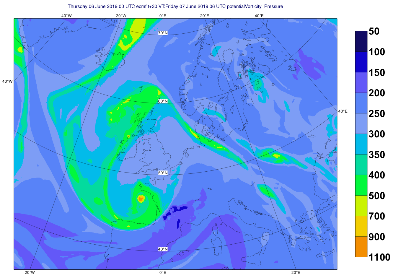

First plot: 30 hour HRES mean sea level pressure forecast
Second plot: Pressure in hPa on surface PV=1.5 PV units, from the same HRES forecast as the first plot, valid at the same time
Third plot: As second plot, but for PV=2 PV units