Getting Data into Metview
Copying files and creating links
By default, Metview can only see files under the $HOME/metview directory. You can select a different home directory for Metview (-u option on the Metview startup command line), but you can also copy files into this directory (or a sub-directory of it) or create links to external data files - this can be useful if you have large data files which would exceed the quota in your home directory.
One way is to do this from a shell command line (ln command), but Metview can also create these links for you.
Right-click an empty spot in the Metview desktop and choose Create New… Link to File and type /home/ectrain/trx/mv_data/ztuv.grb into the File name box (or navigate there and select the file with the mouse). Note that the text label under the new icon is in italics, and there is an arrow in the bottom-left corner - these indicate that this is a link; if you hover the mouse cursor over the icon, the link details will be shown in the status bar. The padlock in the bottom-right corner tells us that this file is read-only. This file contains analysis and 1, 2, 3, 4 and 5-day forecasts for geopotential, temperature and wind at various pressure levels – visualise it to see for yourself.
You can create links to individual files or complete folders. This facility can be used to share folders between users.
Retrieving data from MARS
Metview has the ability to retrieve data directly from the ECMWF MARS archive (or indeed any other MARS archive installed outside ECMWF).
Create a new Mars Retrieval icon. Edit it and set only the following:
| Grid | 1.5/1.5 |
This ensures that the data is transformed onto a regular 1.5 degree grid. Much of Metview's functionality relies on GRIB data being on a grid (regular or quasi-regular) and not stored as spherical harmonics.
If you look at the other parameters in the icon editor, you will see that by default, it will retrieve analysis data (Type = An) of geopotential (Param = Z) on six pressure levels (Levelist = 1000/850/700/500/400/300) for yesterday (Date = -1).
Save the icon, then visualise it. The data should be retrieved, then visualised. From the titles of the different fields in the plot you can confirm that it is the correct data.
We will see in Processing Data how we can manipulate the data returned from MARS.
Icon Feedback
The Mars Retrieval icon gives us the opportunity to explore another feature of Metview. The colour of an icon’s text label tells us which state it is in:
Black | No operation executed since last save (default) |
Orange | Operation in progress, e.g. waiting for data retrieval from database |
Green | Operation successfully executed, data may be cached for some icons |
Red | Operation failed, e.g. due to invalid input parameters |
The icon should currently be green, meaning that if you visualise it (or perform any other action on it), the data will not be retrieved again - the cached copy will be used instead. There are two ways to un-cache the data:
- edit the icon and change at least one parameter (in this case, the cached data will no longer match the retrieval request, so it is deleted)
- right-click on the icon and select Clear result
Use the second technique, then execute the icon and observe as the colour of its name changes.
Icon Output
By now you should have generated some log message, probably when you performed the MARS retrieval. Each icon has its own text output which can be viewed by selecting Log from the icon’s right-click menu. This is only enabled when there is output for that icon, and is reset when the icon’s contents change. Have a look at the log messages for the Mars Retrieval icon (ensure that you have retrieved data first).
You can view a complete history of output from all icons by selecting Log from the Tools menu in any Metview desktop.
For an even more detailed output, you can start Metview on the command line with the ‘-slog’ option - this will write lots of information to your terminal window. This information can be useful when reporting a problem to the Metview team! ‘metview -h’ gives a list of all useful command line options and environment variables.
Field Data in GRIB Files
ECMWF's model output fields are stored in GRIB format, so that is where much of Metview's functionality lies. The following sections will introduce some of the data inspection facilities available.
Examining GRIB Meta-data
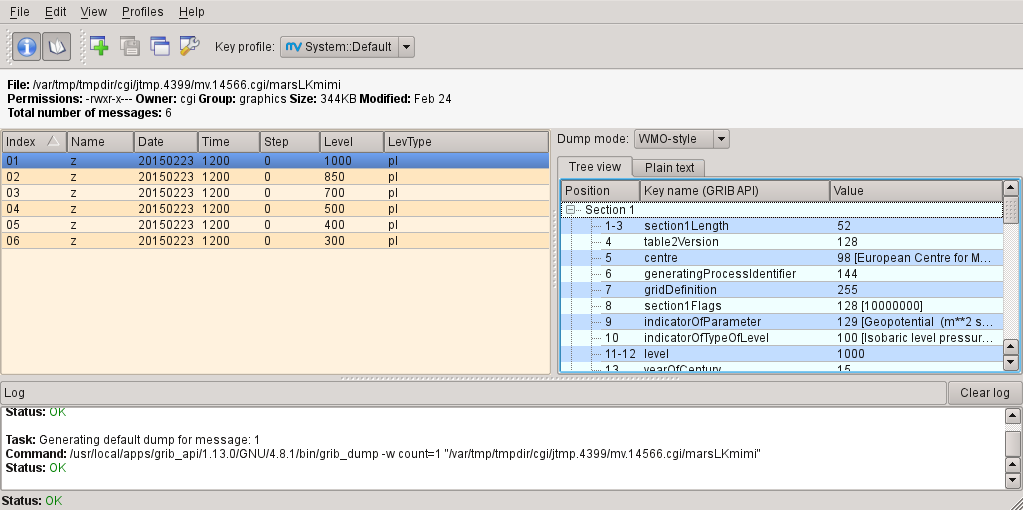
Right-click and Examine the Mars Retrieval icon (if for some reason the retrieval did not work, or you do not have access to MARS, then use ztuv.grb instead).
GRIB file. In this case we have 6 fields (messages) in the file, each represented by a row in the message list on the left-hand side. The right-hand side shows detailed meta-information for the selected message, presented in a number of different ways (try changing between Tree view and Plain text; try different Dump modes). You can sort the fields by clicking on the different column headers. The GRIB Examiner can be customised – see the extra tasks for this chapter, as this is an advanced topic.
Filtering GRIB Data
Metview provides powerful data filtering capabilities. Let’s take our ztuv.grb file and extract the forecast and analysis data separately from it.
![]()
Create a new GRIB Filter icon. This time we’ll rename it from within the icon editor (just to show an alternative way to rename an icon). Edit the icon, and notice the button to the right of the information panel; click it and change the name of the icon to t_3day_fc - we will use this icon to extract only the 3-day forecast data for temperature.
First, we specify the input data. Drag the ztuv.grb icon into the Data field of the editor. This is an icon field – an area where you can drop other icons. Now set the following parameters to extract just the 3-day (72-hour) temperature forecast:
Type | FC or Forecast |
Param | T or Temperature |
Step | 72 |
Visualise this icon and verify that it returns only the data we expect.
Now create a new GRIB Filter icon, rename it t_an and use it to extract only the temperature analysis data:
Type | AN or Analysis |
Param | T or Temperature |
It is quite often the case that GRIB data comes as several fields in the same file, and using the GRIB Filter icon is an easy way to extract just the fields you want without making copies of the file. This icon also has some parameters to perform some post-processing on the data, which we will cover in Processing Data.
Plotting Grid Values

We will now plot the actual grid values. Create a new Contour icon and rename it grid_10x10. Edit it and find the set of parameters close to the bottom of the editor which control the plotting of grid values. Activate grid value plotting, set it to plot both values and markers, and set the lat/lon frequency each to 10. Visualise a scalar field (temperature or geopotential) from ztuv.grb and apply the new visdef icon to it - you will see every 10th grid point plotted. If you wish, you can also deactivate the isolines by setting Conotur to Off.
If you zoom into smaller areas, you may want to see every grid point - duplicate grid_10x10 and call it grid_1x1. Set the lat/lon frequency to 1 - one fast way to do this is to click on the blue ‘revert’ button next to the parameter. This button does two things: it indicates that a parameter has been altered from its default, and it restores the parameter to its default when clicked.
Note that plotting every grid point value for a global plot of a high-resolution field can be slow; it also results in an an readable plot, so it is not recommended!
Cursor Data

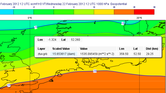
For a closer inspection of data values in a plot without having to apply a special contour icon, the cursor data tool can be used. When activated, the cursor data box follows the mouse cursor around the plot, displaying data for the nearest grid point(s). To ‘dock’ the data box, left-click; to ‘undock’, left-click again and the box will retain its current offset from the cursor. The cursor data tool is available regardless of whether grid value plotting is on or not. Notice that for some parameters it displays both scaled values (as plotted) and the original values (as stored in the data file).
Observation Data in BUFR and Geopoints files
Much observation data is received in BUFR format. BUFR is a complex format, capable of storing almost anything; BUFR files can vary widely, but there are some conventions which can help software to interpret them. We will have a brief overview of Metview's BUFR-handling capabilities here; for more information, see the dedicated tutorial on the Tutorials page.
Examining BUFR Meta-data
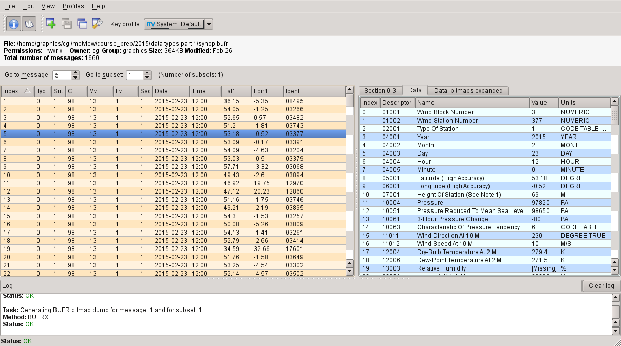
Right-click on the supplied synop.bufr BUFR icon and select examine from the icon menu. This will start the BUFR examiner application. The right-hand panel displays data for the message selected in the left-hand panel. This can be an easy way to find the correct descriptor for a given parameter such as Relative Humidity.
Plotting BUFR Data

Metview is able to plot certain BUFR data directly, mainly some WMO conventional observation types including SYNOP and TEMP.
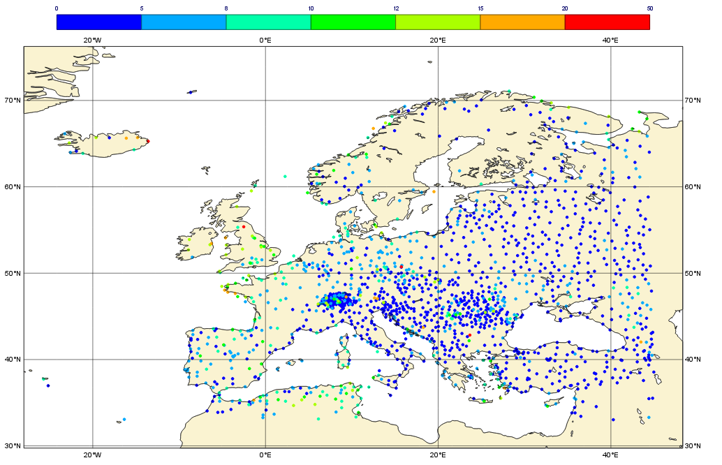
Right-click and visualise the synop.bufr BUFR icon. This will bring up the Display Window using the default visualisation assigned to observation plotting. What we see here is a spatially thinned set of SYNOP observations plotted on the map by using the official WMO-style. If you zoom into a smaller area you will see more observations but the thinning is still kept so that the plot should not seem cluttered.
Filtering Observation Data
BUFR files can contain a lot of information, but we often want to extract just one or two parameters.
The Observation Filter icon extracts a single scalar or vector value from each message in a BUFR file. It is able to perform filtering according to message type, date, time, level, area, location and custom descriptors. Examine the BUFR file and find the descriptor for wind speed at 10m (look in the blue right-hand panel) - make a note of it.
Create a new Observation Filter icon, rename it to wind_speed and edit it. Drop the BUFR icon into the Data field and set the following to extract the wind speed values in geopoints format:
| Output | Geographical Points |
| Parameter | 11012 |
The specifics of the geopoints format are discussed in Data Part 2, but for now just be aware that this is a simple format for storing scattered geographical point data.
Visualise the icon - the filtering will take place, then the result is plotted using the default Symbol Plotting definition, which is to plot the data as numbers. For smaller amounts of data this may be ok, but we can do better. Create a new Symbol Plotting icon and set the following parameters:
| Legend | On |
| Symbol Type | Marker |
| Symbol Table Mode | Advanced |
| Symbol Advanced Table Max Level Colour | Red |
| Symbol Advanced Table Min Level Colour | Blue |
| Symbol Advanced Table Max Colour Direction | Clockwise |
Rename the icon to symb_auto and drop it into the Display Window to see the points coloured according to their value.
Notice that there is a point which claims a wind speed of 80m/s! Reliability can be a big issue with observational data, and this point claims winds of 288km/h! We can filter out data that we consider unrealistic - add the following parameters to your wind_speed icon:
| Custom Filter | Filter By Range |
| Custom Parameter | 11012 |
| Custom Values | 0/50 |
This ensures that we only extract points whose wind speed is between 0 and 50 (m/s). Having a smaller range of values also allows the automatic colour range to spread more evenly through the data. There is still a point with a large value, which you can also filter out if desired.
Notice that the values in the colour scale change as you zoom in and out of different areas - this is computed according to the data currently visible. Try the supplied icon symb_wind_speed_fixed, which has a fixed value/colour mapping.
Extracting vector values from BUFR
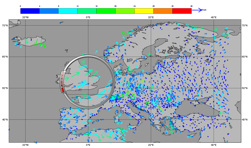
We can extract the wind direction too, and plot the wind as arrows (or flags).
Make a copy of wind_speed and call it wind_speed_and_direction. Find out which descriptor provides wind direction, then change the following parameters in your new filter icon:
| Output | Geographical Polar Vectors |
| Parameter | 11012/11011 |
When you visualise the icon, you will see numbers as before, but if you drop a newly created Wind Plotting icon into the Display Window you will see wind arrows. Try the supplied coloured_wind_arrows icon too. Try changing it to plot wind flags instead of arrows.
You may wish to customise a Coastlines icon to provide a darker background for the plot.
Extra Tasks
Write a macro to plot the wind arrows from BUFR
Use the icons you created to filter and plot the wind arrows from BUFR data to write a macro which produces the same plot. Extract the 'magic numbers' such as the filtering threshold and the wind parameter descriptors into variables at the top of the macro, and use these variables in the macro rather than the raw numbers.
Try the search facilities in the data examiners
Examine the GRIB file and the BUFR file; press CTRL-F to initiate the search. Look carefully at the options!
Create your own GRIB Examiner key profile
When you examine a GRIB file, a list of 'keys' is used to display the GRIB messages - one key per column. These columns are configurable - a 'key profile' is a set of keys, and you can create as many of them as you want. It can be very useful to have different key profiles for different tasks. From the user interface in the GRIB Examiner, create a new key profile; starting either from scratch, or else from a duplicate of the default profile. Note that the Display Window also operates on the same principles, and you can share key profiles between the two.
Observation filtering
Extract 2m temperature values below the freezing point from synop.bufr.
Hints:
- use geopoints output
- use custom filter
- temperature values are given in K