Ongoing analysis Material from: Linus
Discussed in the following Daily reports:
http://intra.ecmwf.int/daily/d/dreport/2013/11/05/sc/
http://intra.ecmwf.int/daily/d/dreport/2013/11/06/sc/
http://intra.ecmwf.int/daily/d/dreport/2013/11/07/sc/

1. Impact
Super-typhoon Haiyan was the third category 5 typhoon to hit the Philippines since 2010. In 2010, Megi made landfall and resulted in 35 people dead and in 2012 Bupha resulted in 1901 dead. The tropical storm seasons in the north-western Pacific is one of the most active and Haiyan was cyclone number 3? and the fifth to made landfall on the Philippines (together with Rumbia, Nari, Utor and Krosa). After making landfall on the Philippines, the cyclone made landfall on the 11 November in southern China and Vietnam.
2. Description of the event
The cyclone formed on the 3 November. On the 6 November 00 UTC the cyclone first classified as a super-typhoon. Late on the 7 November the cyclone made landfall on southern Philippines. Just before (18 UTC) the wind speed was (estimated?) 195 mph.
![]()
MODIS satellite image of Super Typhoon Haiyan taken at 4:25 UTC November 7, 2013. At the time, Haiyan was a Category 5 storm with top winds of 175 mph. The Philippines are visible at the left of the image, and the Caroline Islands at the lower right. Image credit: NASA. Copied from http://www.wunderground.com/blog/JeffMasters/comment.html?entrynum=2572
3. Predictability
3.1 Data assimilation

The figure above shows forecasts of the minimum pressure from long-window 4dvar forecasts, initialised every 12 hour (6 and 18 UTC). In black the estimated (for the hurricane centre at JMA) minimum pressure is plotted. The 12-hour forecast is used as first guess for the next analysis. Especially for the analysis of 7 Nov 18 UTC, the minimum pressure in the analysis is much higher than in the first guess, although the estimate is much lower. The problem here could be that the increments in the data-assimilation is much more large scale that this feature.

This figure shows the same as the previous one but for the e-suite. One difference in the e-suite is the flow-dependent length scale of increments. However, for this case we do not see any big impact of the change.


The figures above shows the MSLP of the first guess and analysis for 7 Nov 18 UTC. This confirms that the cyclone is much more shallow in the analysis.
3.2 HRES
The figure above shows verification of the MSLP fields valid 8 Nov 00 UTC. For high-resolution ps-file, click here. Already the HRES forecast from 10 days before had a cyclone in vicinity of the Philippines. In the forecast from the 3 and 4 November the cyclone starts to be more intense. However, the minimum pressure error is very large (60-70 hPa).
3.3 ENS

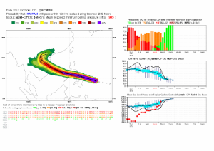

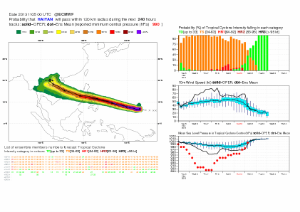
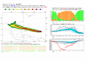
The figures above shows the strike probability product from 8, 7, 6, 5 and 4 November 00 UTC. Here we see a very consistent ensemble regarding the track, but the ensemble has even higher minimum pressure than the HRES.
3.4 Monthly forecasts


Strike probability of a tropical storm for the period 4 to 10 November. forecasts from 4 Nov, 31 Oct, 28 Oct, 24 Oct and 21 October. As expected for above the forecast from 4 November had a high strike probability. For the earlier forecasts there is a risk for a cyclone. However, when checking the climatological occurrences (see figure below), we see that the probabilities are not different from the climatology.

3.5 Comparison with other centres


Control forecasts (from TIGGE) from ECMWF, UKMO, NCEP and JMA. The plots above show MSLP for forecasts initialised 6 Nov 12 UTC and valid 8 Nov 00 UTC.


Control forecasts (from TIGGE) from ECMWF, UKMO, NCEP and JMA. The plots above show MSLP for forecasts initialised 5 Nov 12 UTC and valid 8 Nov 00 UTC.
4. Experience from general performance/other cases
- Megi, Bopha: super-typhoons with far too high minimum pressure
- Francesco: Why did the model produce such a low pressure for Francesco and not for Haiyan?


The figures above shows examples of MSLP of Francesco (left) and Haiyan (right), 36 hours into the forecast. Here we see that Francesco was a much more large-scale system, so the pressure gradients look similar even if Francesco had a minimum pressure of 911 hPa and Haiyan 944 hPa.
5. Good and bad aspects of the forecasts for the event
- Good and consistent forecasts of the track
- Far to high minimum pressure
- Data assimilation made the cyclone less intense?
6. Additional material
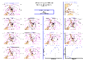
From the WGNE Intercomparison of Tropical Cyclone Track Forecasts, I (Linus) found the following diagnostics of tropical cyclone minimum pressure. The figures below shows scatter plots of observed vs. modelled pressure for the north-western Pactific for the season of 2010. The plots are for ECMWF, UKMO, NCEP and JMA.


For this period, ECMWF seems to have the strongest relation between the observed and modelled depth. The deepest observed typhoon here was Megi with a minimum pressure of less than 900 hPa.For the other centres, NCEP and UKMO have the worst underestimation of the pressure.