-
Created by
 Unknown User (uskh), last updated by Kevin Marsh on Jun 19, 2026
65 minute read
Unknown User (uskh), last updated by Kevin Marsh on Jun 19, 2026
65 minute read
Introduction
Here, we document the ERA5 dataset, which covers the period from January 1940 to the present and continues to be extended forward in near real time. For up to date information on ERA5, please consult the C3S Announcements on the ECMWF forum.
ERA5 is produced using 4D-Var data assimilation and model forecasts in CY41R2 of the ECMWF Integrated Forecast System (IFS), with 137 hybrid sigma/pressure (model) levels in the vertical and the top level at 0.01 hPa. Atmospheric data are available on these levels and they are also interpolated to 37 pressure, 16 potential temperature and 1 potential vorticity level(s) by FULL-POS in the IFS. "Surface or single level" data are also available, containing 2D parameters such as precipitation, top of atmosphere radiation and vertical integrals over the entire depth of the atmosphere. The atmospheric model in the IFS is coupled to a land-surface model (HTESSEL), which produces parameters such as 2m temperature and soil temperatures, and an ocean wave model (WAM), the parameters of which are also designated as "Surface or single level" parameters.
The ERA5 dataset contains one (hourly, 31 km) high resolution realisation (referred to as "reanalysis" or "HRES") and a reduced resolution ten member ensemble (referred to as "ensemble" or "EDA"). The ensemble is required for the data assimilation procedure, but as a by-product also provides an estimate of the relative, random uncertainty. Generally, the data are available at a sub-daily and monthly frequency and consist of analyses and short (18 hour) forecasts, initialised twice daily from analyses at 06 and 18 UTC. Most analysed parameters are also available from the forecasts. However, there are a number of forecast parameters, e.g. mean rates/fluxes and accumulations, that are not available from the analyses.
The data are archived in the ECMWF data archive (MARS) and a pertinent sub-set of the data, interpolated to a regular latitude/longitude grid, has been copied to the C3S Climate Data Store (CDS) disks. On the CDS disks, where single level and pressure level data are available, analyses are provided rather than forecasts, unless the parameter is only available from the forecasts. The interpolation software (MIR) was updated when the ERA5 production was moved to the new ATOS HPC on 24 October 2022.
ERA5.1 is a re-run of ERA5, for the years 2000 to 2006 only, and was produced to improve upon the cold bias in the lower stratosphere seen in ERA5 during this period.
The original ERA5 release contained data from 1979 onwards. The final ERA5 back extension for 1940-1978 has been produced and is available alongside the original/main release.
An ERA5 back extension 1950-1978 (Preliminary version) was produced. Although in many other respects the quality was relatively good, this preliminary data did suffer from excessively intense tropical cyclones. This dataset is now deprecated.
Data update frequency
Initial release data, i.e. data no more than three months behind real time, is called ERA5T.
Both for the CDS and MARS, daily updates for ERA5T are available about 5 days behind real time and monthly mean updates are available about 5 days after the end of the month.
The daily updates for ERA5T data on the CDS occur at no fixed time during the day. However, although it is not guaranteed, the D-5 data are typically available by 12UTC. We are working on reducing the variability of the update time.
For the CDS, ERA5T data for a month is overwritten with the final ERA5 data about two months after the month in question.
For MARS, the final ERA5 data are available about two months after the month in question. In addition, the last few months of data are kept online and can be accessed much quicker than older data on tape.
In the event that serious flaws are detected in ERA5T, the latter could be different to the final ERA5 data. Based on experience with the production of ERA5 so far (and ERA-Interim in the past), our expectation is that such an event would not occur often. So far, it has only occurred once:
- from 1 September to 13 December 2021, the final ERA5 product is different to ERA5T due to the correction of the assimilation of incorrect snow observations in central Asia. Although the differences are mostly limited to that region and mainly to surface parameters, in particular snow depth and soil moisture and to a lesser extent 2m temperature and 2m dewpoint temperature, all the resulting reanalysis fields can differ over the whole globe but should be within their range of uncertainty (which is estimated by the ensemble spread and which can be large for some parameters). On the CDS disks, the initial, ERA5T, fields have been overwritten (with the usual 2-3 month delay), i.e., for these months, access to the original CDS disk, ERA5T product is not possible after it has been overwritten. Potentially incorrect snow observations have been assimilated in ERA5 up to this time, when the effects became noticeable. The quality control of snow observations has been improved in ERA5 from September 2021 and from 15 November 2021 in ERA5T.
- from 1 July to 17 November 2024, the final ERA5 product is different to ERA5T due to the correction of the assimilation of incorrect snow observations on the Alps. The differences are mostly limited to the Alps and mainly to surface parameters (in particular snow depth and 2m temperature and 2m dewpoint temperature). However, all the resulting reanalysis fields do differ slightly over the whole globe but these differences should be within their range of uncertainty (which is estimated by the ensemble spread and which can be large for some parameters).
For the hourly products on CDS disks for both single and pressure levels, some local differences exist between ERA5 and ERA5T for 1 to 24 October 2022 due to a change of the regridding software (MIR) when the ERA5 production was changed from the Cray to ATOS. Differences are not meteorologically significant. For October 2022, there is no difference for the data in native resolution (ERA5-complete).
The IFS and data assimilation
For ERA5, the IFS documentation for CY41R2 should be used.
The twice daily, short (18 hour) forecasts are run from the 06 and 18 UTC analyses.
The 4D-Var data assimilation uses 12 hour windows from 09 UTC to 21 UTC and 21 UTC to 09 UTC (the following day).
The model time step is 12 minutes for the HRES and 20 minutes for the EDA, though occasionally these numbers are adjusted to cope with instabilities.
Data assimilation is a process whereby a model forecast is blended with observations to obtain the best fit to both the forecast and the observations, given the known uncertainties of both. The result is called an analysis (of the state of the atmosphere). For the atmospheric parameters in ERA5, the 4D-Variational (4D-Var) data assimilation windows are 12 hours long, commencing after the first 3 hours of the short forecasts. All the available observations within each 12 hour window are considered by the system, though some might be discarded for various reasons, such as quality control. Some of the parameters under the category "Surface or single level" parameters, are produced by the Land-surface scheme, which uses 1D and 2D Optimal Interpolation and Extended Kalman Filter, data assimilation. The ERA5 MARS archive contains both the analyses and short forecasts. On the CDS disks, where single level and pressure level data are available, analyses are provided rather than forecasts, unless the parameter is only available from the forecasts.
The above data assimilation process, or something similar, is performed for Numerical Weather Prediction (NWP), which provides real time forecasts (and analyses) for many purposes and applications. It would be tempting to use the data produced therein, for climate purposes. However, NWP systems are being improved on a regular basis - typically twice per year at ECMWF. Therefore, the NWP data contain various abrupt changes, due to system improvements, which are mixed in with changes in the climate. Reanalysis avoids this problem by using a fixed NWP system to "re-analyse" the state of the atmosphere for long periods in the past. It should be remembered, however, that spurious changes will still be included in the reanalysis, due to changes in the observing system. The ERA5 data assimilation and forecasting system was used operationally for NWP in 2016. Once this fixed system becomes too old, the reanalysis should be re-done with a more modern, fixed system. Although "reanalysis" suggests that only analyses are provided, the short forecasts are also made available, as noted above.
Data format
Model level parameters are archived in GRIB2 format. All other parameters are in GRIB1 unless otherwise indicated, see Parameter listings.
In the CDS, there is the option of retrieving the data in netCDF format.
For GRIB, ERA5T data can be identified by the key expver=0005 in the GRIB header. ERA5 data is identified by the key expver=0001.
For netCDF data requests which return just ERA5 or just ERA5T data, there is no means of differentiating between ERA5 and ERA5T data in the resulting netCDF files.
For netCDF data requests which return a mixture of ERA5 and ERA5T data, the origin of the variables (1 or 5) will be identifiable in the resulting netCDF files. See this link for more details.
Data organisation and how to download ERA5
The full ERA5 and ERA5T datasets are held in the ECMWF data archive (MARS) and a pertinent sub-set of these data, interpolated to a regular latitude/longitude grid, has been copied to the C3S Climate Data Store (CDS) disks. ERA5.1 is not available from the CDS disks, but is available from MARS (for advice on using ERA5.1 in conjunction with ERA5, CDS data, see "ERA5: mixing CDS and MARS data" in Guidelines). On the CDS disks, where most single level and pressure level parameters are available, analyses are provided rather than forecasts, unless the parameter is only available from the forecasts.
ERA5 (and recent ERA5T) data on the CDS disks can be downloaded either from the relevant CDS download page or using the CDS API.
Getting data from the CDS disks provides the fastest access to ERA5.
ERA5 data in MARS can be accessed using the CDS API, but access is relatively slow.
Documentation is available on How to download ERA5.
Date and time specification
In MARS: the date and time of the data is specified with three MARS keywords: date, time and (forecast) step. For analyses, step=0 hours so that date and time specify the analysis date/time. For forecasts, date and time specify the forecast start time and step specifies the number of hours since that start time. The combination of date, time and step defines the validity date/time. For analyses, the validity date/time is equal to the analysis date/time.
In the CDS: analyses are provided rather than forecasts, unless the parameter is only available from the forecasts. The date and time of the data is specified using the validity date/time, so step does not need to be specified. For forecasts, steps between 1 and 12 hours have been used to provide data for all the validity times in each 24 hours, see Table 0 below.
Temporal frequency
For sub-daily data for the HRES (stream=oper/wave) the analyses (type=an) are available hourly. The short forecasts, run twice daily from 06 and 18 UTC, provide hourly output forecast steps from 0 to 18 hours (only steps 1 to 12 hours are available on the CDS disks). For the EDA, the sub-daily non-wave data (stream=enda) are available every 3 hours but the sub-daily wave data (stream=ewda) are available hourly in MARS and 3 hourly on the CDS disks.
Spatial grid
The ERA5 HRES atmospheric data has a resolution of 31km, 0.28125 degrees, and the EDA has a resolution of 63km, 0.5625 degrees. (Depending on the parameter, the data are archived either as spectral coefficients with a triangular truncation of T639 (HRES) and T319 (EDA) or on a reduced Gaussian grid with a resolution of N320 (HRES) and N160 (EDA). These grids are so called "linear grids", sometimes referred to as TL639 (HRES) and TL319 (EDA).)
The wave data are produced and archived on a different grid to that of the atmospheric model, namely a reduced latitude/longitude grid with a resolution of 0.36 degrees (HRES) and 1.0 degree (EDA).
ERA5 data available from the CDS disks has been pre-interpolated to a regular latitude/longitude grid appropriate for that data.
The interpolation method is based on the MIR software. For the production on the Cray HPC (1 January 1940 to 24 October 2022 inclusive) this was an early version of MIR, while for the production on ATOS (25 October 2022 onwards) this is based on the MIR version of the ECMWF MARS client. Differences between both versions are in general small, very localized and not meteorologically significant. For data on pressure levels, differences are mainly limited to the exact north and south pole (90N and 90S). For single-level data, for some fields there are differences at the poles as well, while for some other fields, there are additional sets of isolated points with differences. In both cases this represents an improvement of the interpolation software.
The article Model grid box and time step might be useful.
Surface elevation datasets used by ERA5
In order to define the surface geopotential in ERA5, the IFS uses surface elevation data interpolated from a combination of SRTM30 and other surface elevation datasets. For more details please see the IFS documentation, Cycle 41r2, Part IV. Physical processes, section 11.2.2 Surface elevation data at 30 arc seconds.
Spatial reference systems and Earth model
The IFS assumes that the underlying shape of the Earth is a perfect sphere, of radius 6371.229 km, with the surface elevation specified relative to that sphere. The geodetic latitude/longitude of the surface elevation datasets are used as if they were the spherical latitude/longitude of the IFS.
ERA5 data is referenced in the horizontal with respect to the WGS84 ellipse (which defines the major/minor axes) and in the vertical it is referenced to the EGM96 geoid over land but over ocean it is referenced to mean sea level, with the approximation that this is assumed to be coincident with the geoid. For more information on the relationship between mean sea level and the geoid, see for example Gregory et al. (2019).
For data in GRIB1 format the earth model is a sphere with radius = 6367.47 km (note, this is inconsistent with what is actually used in the IFS), as defined in the WMO GRIB Edition 1 specifications, Table 7, GDS Octet 17.
For data in GRIB2 format the earth model is a sphere with radius = 6371.229 km (note, this is consistent with what is actually used in the IFS), as defined in the WMO GRIB2 specifications, section 2.2.1, Code Table 3.2, Code figure 6.
For data in NetCDF format (i.e. converted from the native GRIB format to NetCDF), the earth model is inherited from the GRIB data.
Production experiments
In order to speed up production, the historic ERA5 data was produced by running several parallel experiments which were then spliced together to form the final product.
A discontinuity can occur at the transition between the different experiments. Please see the Known issues for an example. The degree of discontinuity depends on how well the experiments were "spun-up". How well "spun-up" an experiment is, depends on the initial, chosen, state of the atmosphere and land surface at the beginning of the experiment, how long the experiment is run for, before being used for production, and the parameter(s) of interest - some parameters, such as those for the deeper soil and for the higher atmospheric levels, take longer to spin-up than others.
The information below gives the date ranges for the various production experiments (and hence the transition points) for the final version of ERA5 and also indicates when the computing system changed from the Cray to the ATOS.
Note, that forecasts start from the relevant analysis at the forecast start date/time, so the provenance of the whole of each forecast is the same as that of the analysis at the forecast start date/time.
Accuracy and uncertainty
ERA5 is produced using 4D-Var data assimilation and model forecasts in CY41R2 of the IFS. The 4D-Var in ERA5 utilises 12 hour assimilation windows from 9-21 UTC and 21-9 UTC, where the background forecast and all the observations falling within a time window are used to specify all the analyses during that window. However, the accuracy of the analyses is not uniform throughout each window. If the model and observations are unbiased and their errors follow Gaussian distributions and if the observations are homogeneous in space and time, then the analysis error will be smallest in the middle of the assimilation window. However, because none of these assumptions are actually true in the IFS, the particular parameter and location of interest are important, too. Knowing that, a careful study should show at which points during the assimilation windows the analysis is most accurate.
The 10 member ensemble is required for the data assimilation procedure. However, as a useful by-product, this ensemble also provides an estimate of the relative, random uncertainty. The "spread" of the 10 member ensemble, encapsulated by the standard deviation, provides a measure of this uncertainty and is larger for time periods and spatial locations where the uncertainty is relatively large and is smaller when and where there is more certainty in the analysed/forecast values. The spread is a measure of the relative uncertainty, so the numbers do not provide the absolute uncertainty. On the whole, the uncertainty becomes larger as you go back in time, when the observing system was not as good as in the present day, and in data sparse locations such as the pre-satellite era, southern hemisphere. In general, apart from that for the sea surface temperature, the spread does not represent systematic uncertainty, only random, or "synoptic", uncertainty. For more information, see ERA5: uncertainty estimation.
Instantaneous parameters
All the analysed parameters and many of the forecast parameters are described as "instantaneous". For more information on what instantaneous means, see Parameters valid at the specified time. Such instantaneous parameters may, or may not, have been averaged in time, to produce monthly means.
Mean rates/fluxes and accumulations
Such parameters, which are only available from forecasts, have undergone particular types of statistical processing (temporal mean or accumulation, respectively) over a period of time called the processing period. In addition, these parameters may, or may not, have been averaged in time, to produce monthly means.
The accumulations (over the accumulation/processing period) in the short forecasts (from 06 and 18 UTC) of ERA5 are treated differently compared with those in ERA-Interim and operational data (where the accumulations are from the beginning of the forecast to the validity date/time). In the short forecasts of ERA5, the accumulations are since the previous post processing (archiving), so for:
- reanalysis: accumulations are over the hour (the accumulation/processing period) ending at the validity date/time
- ensemble: accumulations are over the 3 hours (the accumulation/processing period) ending at the validity date/time
- Monthly means (of daily means, stream=moda/edmo): accumulations have been scaled to have an "effective" processing period of one day, see section Monthly means
Mean rate/flux parameters in ERA5 (e.g. Table 4 for surface and single levels) provide similar information to accumulations (e.g. Table 3 for surface and single levels), except they are expressed as temporal means, over the same processing periods, and so have units of "per second".
- Mean rate/flux parameters are easier to deal with than accumulations because the units do not vary with the processing period.
- The mean rate hydrological parameters (e.g. the "Mean total precipitation rate") have units of "kg m-2 s-1", which are equivalent to "mm s-1". They can be multiplied by 86400 seconds (24 hours) to convert to kg m-2 day-1 or mm day-1.
Note that:
- For the CDS time, or validity time, of 00 UTC, the mean rates/fluxes and accumulations are over the hour (3 hours for the EDA) ending at 00 UTC i.e. the mean or accumulation is during part of the previous day.
- Mean rates/fluxes and accumulations are not available from the analyses.
- Mean rates/fluxes and accumulations at step=0 have values of zero because the length of the processing period is zero.
Minimum/maximum since the previous post processing
The short forecasts of ERA5 contain some surface and single level parameters that are the minimum or maximum value since the previous post processing (archiving), see Table 5 below. So, for:
- reanalysis: the minimum or maximum values are in the hour (the processing period) ending at the validity date/time
- ensemble: the minimum or maximum values are in the 3 hours (the processing period) ending at the validity date/time
Wave spectra
The ocean wave model used in ERA5 (WAM, which is included in the IFS) provides wave spectra with 24 directions and 30 frequencies (see "2D wave spectra (single)", Table 7).
Monthly means
In addition to the sub-daily data, most analysed and forecast parameters are also available as monthly means. For the surface and single level parameters, there are some exceptions which are listed in Table 8.
Monthly means are available in two forms:
- Synoptic monthly means, for each particular time and forecast step (stream=mnth/wamo/edmm/ewmm) - in the CDS, referred to as "monthly averaged by hour of day".
- Monthly means (of daily means, stream=moda/wamd/edmo/ewmo) for the month as a whole - in the CDS, referred to as "monthly averaged". These monthly means are created from all the hourly (3 hourly for the ensemble) data in the month.
Monthly means for:
- forecast parameters are created using the first 12 hours of the twice daily short forecasts (beginning at 06 and 18 UTC).
- analysis and instantaneous forecast parameters are created from data with a validity time in the month, between 00 and 23 UTC, which excludes the time 00 UTC on the first day of the following month.
- accumulation and mean rate/flux forecast parameters are created from data with processing periods that fall within the month.
- monthly means of daily means, for accumulations and mean rates/fluxes are created from contiguous data with processing periods spanning from 00 UTC on the first day of the month to 00 UTC on the first day of the following month i.e. they are accumulations or mean rates/fluxes for the complete, whole month.
The accumulations in monthly means (of daily means, stream=moda/edmo) have been scaled to have an "effective" processing period of one day, so for accumulations in these streams:
- The hydrological parameters have effective units of "m of water per day" and so they should be multiplied by 1000 to convert to kgm-2day-1 or mmday-1.
- The energy (turbulent and radiative) and momentum fluxes should be divided by 86400 seconds (24 hours) to convert to the commonly used units of Wm-2 and Nm-2, respectively.
The monthly data in the CDS under 'ERA5 monthly averaged data' has been created by first creating monthly data on the native grid, then regridding this to the lat-lon grid used in the CDS. The hourly data in the CDS under 'ERA5 hourly data' has been created by regridding from the native to the lat-lon grid. Any calculation of monthly means using this hourly data takes place on the already regridded dataset.
In general, the monthly means calculated from the hourly data, or provided in the CDS should be identical, as regridding and averaging are both linear operations. However, when calculating wind speed, there is a nonlinear transformation sqrt(u*u+v*v) in between and then the order does matter. Therefore, small differences can be seen where the wind fields themselves vary quickly with location, like going from sea to the high volcanos over Hawaii.
Ensemble means and standard deviations
For the EDA sub-daily data (stream=enda/ewda), compared with HRES sub-daily data (stream=oper/wave), ensemble means and standard deviations (type=em/es) are also available. Both these quantities are calculated from all the 10-members (i.e., including the control).
Ensemble standard deviation is often referred to as ensemble spread and is calculated with respect to the ensemble mean. The ensemble standard deviation is not the sample stdv, so we divide by 10 rather than 9 (N-1).
Ensemble means and standard deviations contain analysed parameters when step=0, otherwise they contain forecast parameters. However, only surface and pressure level data (levtype=sfc/pl) contain forecast steps beyond 3 hours. There are no monthly means for ensemble means and standard deviations.
Level listings
Pressure levels (hPa): 1000/975/950/925/900/875/850/825/800/775/750/700/650/600/550/500/450/400/350/300/250/225/200/175/150/125/100/70/50/30/20/10/7/5/3/2/1
Potential temperature levels (K): 265/275/285/300/315/320/330/350/370/395/430/475/530/600/700/850
Potential vorticity level (10-9 K m2 kg-1 s-1 or 10-3 PVU): 2000 (which is representative of the dynamical tropopause)
Model levels: 1/to/137, which are described at L137 model level definitions and ERA5: compute pressure and geopotential on model levels, geopotential height and geometric height. The model levels are hybrid pressure/sigma. For more information, see the documentation of the underlying model, ECMWF's IFS, CY41R2, Part III. Dynamics and numerical procedures, Chapter 2 Basic equations and discretisation.
Parameter listings
Tables 1-6 below describe the surface and single level parameters (levtype=sfc), Table 7 describes wave parameters, Table 8 describes the monthly mean exceptions for surface and single level and wave parameters and Tables 9-13 describe upper air parameters on various levtypes.
Information on all ECMWF parameters (e.g. columns shortName and paramId) is available from the ECMWF parameter database
Please note that with the release of the latest version of ecCodes, some shortNames names have changed. As a result, some of the shortNames in the tables below will need to be updated. Until this is completed, please use the relevant entry in the parameter database as official reference for the shortNames and names.
Table 1: surface and single level parameters: invariants (in time)
(stream=oper/enda/mnth/moda/edmm/edmo, levtype=sfc)
(The native grid is the reduced Gaussian grid N320 (N160 for the EDA))
count | name | units | Variable name in CDS | shortName | paramId | an | fc |
|---|---|---|---|---|---|---|---|
1 | (0 - 1) | lake_cover | cl | 26 | x | x | |
2 | m | lake_depth | dl | 228007 | x | x | |
3 | (0 - 1) | low_vegetation_cover | cvl | 27 | x | ||
4 | (0 - 1) | high_vegetation_cover | cvh | 28 | x | ||
5 | ~ | type_of_low_vegetation | tvl | 29 | x | ||
6 | ~ | type_of_high_vegetation | tvh | 30 | x | ||
7 | ~ | soil_type | slt | 43 | x | ||
8 | m | standard_deviation_of_filtered_subgrid_orography | sdfor | 74 | x | ||
9 | m**2 s**-2 | geopotential | z | 129 | x | x | |
10 | ~ | standard_deviation_of_orography | sdor | 160 | x | ||
11 | ~ | anisotropy_of_sub_gridscale_orography | isor | 161 | x | ||
12 | radians | angle_of_sub_gridscale_orography | anor | 162 | x | ||
13 | ~ | slope_of_sub_gridscale_orography | slor | 163 | x | ||
14 | (0 - 1) | land_sea_mask | lsm | 172 | x | x |
1Soil type (texture) determines the saturation, field capacity and permanent wilting point at all the soil levels, see Table 8.9 in Chapter 8 Surface parametrization, Part IV Physical Processes of the IFS documentation (CY41R2 for ERA5).
Table 2: surface and single level parameters: instantaneous
(stream=oper/enda/mnth/moda/edmm/edmo, levtype=sfc)
(The native grid is the reduced Gaussian grid N320 (N160 for the EDA))
count | name | units | Variable name in CDS | shortName | paramId | an | fc |
|---|---|---|---|---|---|---|---|
1 | J kg**-1 | convective_inhibition | cin | 228001 | x | ||
2 | m s**-1 | friction_velocity | zust | 228003 | x | ||
3 | K | lake_mix_layer_temperature | lmlt | 228008 | x | x | |
4 | m | lake_mix_layer_depth | lmld | 228009 | x | x | |
5 | K | lake_bottom_temperature | lblt | 228010 | x | x | |
6 | K | lake_total_layer_temperature | ltlt | 228011 | x | x | |
7 | dimensionless | lake_shape_factor | lshf | 228012 | x | x | |
8 | K | lake_ice_temperature | lict | 228013 | x | x | |
9 | m | lake_ice_depth | licd | 228014 | x | x | |
10 | (0 - 1) | uv_visible_albedo_for_direct_radiation | aluvp | 15 | x | x | |
11 | Minimum vertical gradient of refractivity inside trapping layer | m**-1 | minimum_vertical_gradient_of_refractivity_inside_trapping_layer | dndzn | 228015 | x | |
12 | (0 - 1) | uv_visible_albedo_for_diffuse_radiation | aluvd | 16 | x | x | |
13 | Mean vertical gradient of refractivity inside trapping layer | m**-1 | mean_vertical_gradient_of_refractivity_inside_trapping_layer | dndza | 228016 | x | |
14 | (0 - 1) | near_ir_albedo_for_direct_radiation | alnip | 17 | x | x | |
15 | m | duct_base_height | dctb | 228017 | x | ||
16 | (0 - 1) | near_ir_albedo_for_diffuse_radiation | alnid | 18 | x | x | |
17 | m | trapping_layer_base_height | tplb | 228018 | x | ||
18 | m | trapping_layer_top_height | tplt | 228019 | x | ||
19 | m | cloud_base_height | cbh | 228023 | x | ||
20 | m | zero_degree_level | deg0l | 228024 | x | ||
21 | m s**-1 | instantaneous_10m_wind_gust | i10fg | 228029 | x | ||
22 | (0 - 1) | sea-ice_cover | ci | 31 | x | x | |
23 | (0 - 1) | snow_albedo | asn | 32 | x | x | |
24 | kg m**-3 | snow_density | rsn | 33 | x | x | |
25 | K | sea_surface_temperature | sst | 34 | x | x | |
26 | K | ice_temperature_layer_1 | istl1 | 35 | x | x | |
27 | K | ice_temperature_layer_2 | istl2 | 36 | x | x | |
28 | K | ice_temperature_layer_3 | istl3 | 37 | x | x | |
29 | K | ice_temperature_layer_4 | istl4 | 38 | x | x | |
30 | m**3 m**-3 | volumetric_soil_water_layer_1 | swvl1 | 39 | x | x | |
31 | m**3 m**-3 | volumetric_soil_water_layer_2 | swvl2 | 40 | x | x | |
32 | m**3 m**-3 | volumetric_soil_water_layer_3 | swvl3 | 41 | x | x | |
33 | m**3 m**-3 | volumetric_soil_water_layer_4 | swvl4 | 42 | x | x | |
34 | J kg**-1 | convective_available_potential_energy | cape | 59 | x | x | |
35 | m**2 m**-2 | leaf_area_index_low_vegetation | lai_lv | 66 | x | x | |
36 | m**2 m**-2 | leaf_area_index_high_vegetation | lai_hv | 67 | x | x | |
37 | m s**-1 | 10m_u-component_of_neutral_wind | u10n | 228131 | x | x | |
38 | m s**-1 | 10m_v-component_of_neutral_wind | v10n | 228132 | x | x | |
39 | Pa | surface_pressure | sp | 134 | x | x | |
40 | K | soil_temperature_level_1 | stl1 | 139 | x | x | |
41 | m of water equivalent | snow_depth | sd | 141 | x | x | |
42 | ~ | charnock | chnk | 148 | x | x | |
43 | Pa | mean_sea_level_pressure | msl | 151 | x | x | |
44 | m | boundary_layer_height | blh | 159 | x | x | |
45 | (0 - 1) | total_cloud_cover | tcc | 164 | x | x | |
46 | m s**-1 | 10m_u_component_of_wind | 10u | 165 | x | x | |
47 | m s**-1 | 10m_v_component_of_wind | 10v | 166 | x | x | |
48 | K | 2m_temperature | 2t | 167 | x | x | |
49 | K | 2m_dewpoint_temperature | 2d | 168 | x | x | |
50 | K | soil_temperature_level_2 | stl2 | 170 | x | x | |
51 | K | soil_temperature_level_3 | stl3 | 183 | x | x | |
52 | (0 - 1) | low_cloud_cover | lcc | 186 | x | x | |
53 | (0 - 1) | medium_cloud_cover | mcc | 187 | x | x | |
54 | (0 - 1) | high_cloud_cover | hcc | 188 | x | x | |
55 | m of water equivalent | skin_reservoir_content | src | 198 | x | x | |
56 | (0 - 1) | instantaneous_large_scale_surface_precipitation_fraction | ilspf | 228217 | x | ||
57 | kg m**-2 s**-1 | convective_rain_rate | crr | 228218 | x | ||
58 | kg m**-2 s**-1 | large_scale_rain_rate | lsrr | 228219 | x | ||
59 | kg m**-2 s**-1 | convective_snowfall_rate_water_equivalent | csfr | 228220 | x | ||
60 | kg m**-2 s**-1 | large_scale_snowfall_rate_water_equivalent | lssfr | 228221 | x | ||
61 | N m**-2 | instantaneous_eastward_turbulent_surface_stress | iews | 229 | x | x | |
62 | N m**-2 | instantaneous_northward_turbulent_surface_stress | inss | 230 | x | x | |
63 | W m**-2 | instantaneous_surface_sensible_heat_flux | ishf | 231 | x | x | |
64 | kg m**-2 s**-1 | instantaneous_moisture_flux | ie | 232 | x | x | |
65 | K | skin_temperature | skt | 235 | x | x | |
66 | K | soil_temperature_level_4 | stl4 | 236 | x | x | |
67 | K | temperature_of_snow_layer | tsn | 238 | x | x | |
68 | (0 - 1) | forecast_albedo | fal | 243 | x | x | |
69 | m | forecast_surface_roughness | fsr | 244 | x | x | |
70 | ~ | forecast_logarithm_of_surface_roughness_for_heat | flsr | 245 | x | x | |
71 | m s**-1 | 100m_u_component_of_wind | 100u | 228246 | x | x | |
72 | m s**-1 | 100m_v_component_of_wind | 100v | 228247 | x | x | |
73 | code table (4.201) | precipitation_type | ptype | 260015 | x | ||
74 | K | k_index | kx | 260121 | x | ||
75 | K | total_totals_index | totalx | 260123 | x |
2GRIB2 format
3Leaf Area Index (LAI) parameters are based on a monthly climatology. Users will only see monthly variability, but not inter-annual variability.
Table 3: surface and single level parameters: accumulations
(stream=oper/enda/mnth/moda/edmm/edmo, levtype=sfc)
(The native grid is the reduced Gaussian grid N320 (N160 for the EDA))
count | name | units | Variable name in CDS | shortName | paramId | an | fc |
|---|---|---|---|---|---|---|---|
1 | s | large_scale_precipitation_fraction | lspf | 50 | x | ||
2 | J m**-2 | downward_uv_radiation_at_the_surface | uvb | 57 | x | ||
3 | J m**-2 | boundary_layer_dissipation | bld | 145 | x | ||
4 | J m**-2 | surface_sensible_heat_flux | sshf | 146 | x | ||
5 | J m**-2 | surface_latent_heat_flux | slhf | 147 | x | ||
6 | J m**-2 | surface_solar_radiation_downwards | ssrd | 169 | x | ||
7 | J m**-2 | surface_thermal_radiation_downwards | strd | 175 | x | ||
8 | J m**-2 | surface_net_solar_radiation | ssr | 176 | x | ||
9 | J m**-2 | surface_net_thermal_radiation | str | 177 | x | ||
10 | J m**-2 | top_net_solar_radiation | tsr | 178 | x | ||
11 | J m**-2 | top_net_thermal_radiation | ttr | 179 | x | ||
12 | N m**-2 s | eastward_turbulent_surface_stress | ewss | 180 | x | ||
13 | N m**-2 s | northward_turbulent_surface_stress | nsss | 181 | x | ||
14 | N m**-2 s | eastward_gravity_wave_surface_stress | lgws | 195 | x | ||
15 | N m**-2 s | northward_gravity_wave_surface_stress | mgws | 196 | x | ||
16 | J m**-2 | gravity_wave_dissipation | gwd | 197 | x | ||
17 | J m**-2 | top_net_solar_radiation_clear_sky | tsrc | 208 | x | ||
18 | J m**-2 | top_net_thermal_radiation_clear_sky | ttrc | 209 | x | ||
19 | J m**-2 | surface_net_solar_radiation_clear_sky | ssrc | 210 | x | ||
20 | J m**-2 | surface_net_thermal_radiation_clear_sky | strc | 211 | x | ||
21 | J m**-2 | toa_incident_solar_radiation | tisr | 212 | x | ||
22 | kg m**-2 | vertically_integrated_moisture_divergence | vimd | 213 | x | ||
23 | J m**-2 | total_sky_direct_solar_radiation_at_surface | fdir | 228021 | x | ||
24 | J m**-2 | clear_sky_direct_solar_radiation_at_surface | cdir | 228022 | x | ||
25 | J m**-2 | surface_solar_radiation_downward_clear_sky | ssrdc | 228129 | x | ||
26 | J m**-2 | surface_thermal_radiation_downward_clear_sky | strdc | 228130 | x | ||
27 | m | surface_runoff | sro | 8 | x | ||
28 | m | sub_surface_runoff | ssro | 9 | x | ||
29 | m of water equivalent | snow_evaporation | es | 44 | x | ||
30 | m of water equivalent | snowmelt | smlt | 45 | x | ||
31 | m | large_scale_precipitation | lsp | 142 | x | ||
32 | m | convective_precipitation | cp | 143 | x | ||
33 | m of water equivalent | snowfall | sf | 144 | x | ||
34 | m of water equivalent | evaporation | e | 182 | x | ||
35 | m | runoff | ro | 205 | x | ||
36 | m | total_precipitation | tp | 228 | x | ||
37 | m of water equivalent | convective_snowfall | csf | 239 | x | ||
38 | m of water equivalent | large_scale_snowfall | lsf | 240 | x | ||
39 | m | potential_evaporation | pev | 228251 | x |
The accumulations in monthly means of daily means (stream=moda/edmo), see monthly means, have been scaled to have units that include "per day", so for accumulations in these streams:
- Most hydrological parameters are in units of "m of water per day", so these should be multiplied by 1000 to convert to kg m-2 day-1 or mm day-1.
- Energy (turbulent and radiative) and momentum fluxes should be divided by 86400 seconds (24 hours) to convert to the commonly used units of W m-2 and N m-2, respectively.
Table 4: surface and single level parameters: mean rates/fluxes
(stream=oper/enda/mnth/moda/edmm/edmo, levtype=sfc)
(The native grid is the reduced Gaussian grid N320 (N160 for the EDA))
| count | name | units | Variable name in CDS | shortName | paramId | an | fc |
|---|---|---|---|---|---|---|---|
| 1 | kg m**-2 s**-1 | mean_surface_runoff_rate | msror | 235020 | x | ||
| 2 | kg m**-2 s**-1 | mean_sub_surface_runoff_rate | mssror | 235021 | x | ||
| 3 | kg m**-2 s**-1 | mean_snow_evaporation_rate | mser | 235023 | x | ||
| 4 | kg m**-2 s**-1 | mean_snowmelt_rate | msmr | 235024 | x | ||
| 5 | Proportion | mean_large_scale_precipitation_fraction | mlspf | 235026 | x | ||
| 6 | W m**-2 | mean_surface_downward_uv_radiation_flux | msdwuvrf | 235027 | x | ||
| 7 | kg m**-2 s**-1 | mean_large_scale_precipitation_rate | mlspr | 235029 | x | ||
| 8 | kg m**-2 s**-1 | mean_convective_precipitation_rate | mcpr | 235030 | x | ||
| 9 | kg m**-2 s**-1 | mean_snowfall_rate | msr | 235031 | x | ||
| 10 | W m**-2 | mean_boundary_layer_dissipation | mbld | 235032 | x | ||
| 11 | W m**-2 | mean_surface_sensible_heat_flux | msshf | 235033 | x | ||
| 12 | W m**-2 | mean_surface_latent_heat_flux | mslhf | 235034 | x | ||
| 13 | W m**-2 | mean_surface_downward_short_wave_radiation_flux | msdwswrf | 235035 | x | ||
| 14 | W m**-2 | mean_surface_downward_long_wave_radiation_flux | msdwlwrf | 235036 | x | ||
| 15 | W m**-2 | mean_surface_net_short_wave_radiation_flux | msnswrf | 235037 | x | ||
| 16 | W m**-2 | mean_surface_net_long_wave_radiation_flux | msnlwrf | 235038 | x | ||
| 17 | W m**-2 | mean_top_net_short_wave_radiation_flux | mtnswrf | 235039 | x | ||
| 18 | W m**-2 | mean_top_net_long_wave_radiation_flux | mtnlwrf | 235040 | x | ||
| 19 | N m**-2 | mean_eastward_turbulent_surface_stress | metss | 235041 | x | ||
| 20 | N m**-2 | mean_northward_turbulent_surface_stress | mntss | 235042 | x | ||
| 21 | kg m**-2 s**-1 | mean_evaporation_rate | mer | 235043 | x | ||
| 22 | N m**-2 | mean_eastward_gravity_wave_surface_stress | megwss | 235045 | x | ||
| 23 | N m**-2 | mean_northward_gravity_wave_surface_stress | mngwss | 235046 | x | ||
| 24 | W m**-2 | mean_gravity_wave_dissipation | mgwd | 235047 | x | ||
| 25 | kg m**-2 s**-1 | mean_runoff_rate | mror | 235048 | x | ||
| 26 | W m**-2 | mean_top_net_short_wave_radiation_flux_clear_sky | mtnswrfcs | 235049 | x | ||
| 27 | W m**-2 | mean_top_net_long_wave_radiation_flux_clear_sky | mtnlwrfcs | 235050 | x | ||
| 28 | W m**-2 | mean_surface_net_short_wave_radiation_flux_clear_sky | msnswrfcs | 235051 | x | ||
| 29 | W m**-2 | mean_surface_net_long_wave_radiation_flux_clear_sky | msnlwrfcs | 235052 | x | ||
| 30 | W m**-2 | mean_top_downward_short_wave_radiation_flux | mtdwswrf | 235053 | x | ||
| 31 | kg m**-2 s**-1 | mean_vertically_integrated_moisture_divergence | mvimd | 235054 | x | ||
| 32 | kg m**-2 s**-1 | mean_total_precipitation_rate | mtpr | 235055 | x | ||
| 33 | kg m**-2 s**-1 | mean_convective_snowfall_rate | mcsr | 235056 | x | ||
| 34 | kg m**-2 s**-1 | mean_large_scale_snowfall_rate | mlssr | 235057 | x | ||
| 35 | W m**-2 | mean_surface_direct_short_wave_radiation_flux | msdrswrf | 235058 | x | ||
| 36 | W m**-2 | mean_surface_direct_short_wave_radiation_flux_clear_sky | msdrswrfcs | 235059 | x | ||
| 37 | W m**-2 | mean_surface_downward_short_wave_radiation_flux_clear_sky | msdwswrfcs | 235068 | x | ||
| 38 | W m**-2 | mean_surface_downward_long_wave_radiation_flux_clear_sky | msdwlwrfcs | 235069 | x | ||
| 39 | kg m**-2 s**-1 | mean_potential_evaporation_rate | mper | 235070 | x |
The mean rates/fluxes in Table 4 provide similar information to the accumulations in Table 3, except they are expressed as temporal averages, and so have units of "per second". The mean rate hydrological parameters have units of "kg m-2 s-1" and so they can be multiplied by 86400 seconds (24 hours) to convert to kg m-2 day-1 or mm day-1.
Table 5: surface and single level parameters: minimum/maximum
(stream=oper/enda, levtype=sfc)
(The native grid is the reduced Gaussian grid N320 (N160 for the EDA))
count | name | units | Variable name in CDS | shortName | paramId | an | fc |
|---|---|---|---|---|---|---|---|
1 | m s**-1 | 10m_wind_gust_since_previous_post_processing | 10fg | 49 | x | ||
2 | Maximum temperature at 2 metres since previous post-processing | K | maximum_2m_temperature_since_previous_post_processing | mx2t | 201 | x | |
3 | Minimum temperature at 2 metres since previous post-processing | K | minimum_2m_temperature_since_previous_post_processing | mn2t | 202 | x | |
4 | Maximum total precipitation rate since previous post-processing | kg m**-2 s**-1 | maximum_total_precipitation_rate_since_previous_post_processing | mxtpr | 228226 | x | |
5 | Minimum total precipitation rate since previous post-processing | kg m**-2 s**-1 | minimum_total_precipitation_rate_since_previous_post_processing | mntpr | 228227 | x |
Table 6: surface and single level parameters: vertical integrals and total column: instantaneous
(stream=oper/enda/mnth/moda/edmm/edmo, levtype=sfc - vertical integrals not available for type=em/es
(The native grid is the reduced Gaussian grid N320 (N160 for the EDA))
count | name | units | Variable name in CDS | shortName | paramId | an | fc |
|---|---|---|---|---|---|---|---|
1 | kg m**-2 | vertical_integral_of_mass_of_atmosphere | vima | 162053 | x | x | |
2 | K kg m**-2 | vertical_integral_of_temperature | vit | 162054 | x | x | |
3 | J m**-2 | vertical_integral_of_kinetic_energy | vike | 162059 | x | x | |
4 | J m**-2 | vertical_integral_of_thermal_energy | vithe | 162060 | x | x | |
5 | J m**-2 | vertical_integral_of_potential_and_internal_energy | vipie | 162061 | x | x | |
6 | J m**-2 | vertical_integral_of_potential_internal_and_latent_energy | vipile | 162062 | x | x | |
7 | J m**-2 | vertical_integral_of_total_energy | vitoe | 162063 | x | x | |
8 | W m**-2 | vertical_integral_of_energy_conversion | viec | 162064 | x | x | |
9 | kg m**-1 s**-1 | vertical_integral_of_eastward_mass_flux | vimae | 162065 | x | x | |
10 | kg m**-1 s**-1 | vertical_integral_of_northward_mass_flux | viman | 162066 | x | x | |
11 | W m**-1 | vertical_integral_of_eastward_kinetic_energy_flux | vikee | 162067 | x | x | |
12 | W m**-1 | vertical_integral_of_northward_kinetic_energy_flux | viken | 162068 | x | x | |
13 | W m**-1 | vertical_integral_of_eastward_heat_flux | vithee | 162069 | x | x | |
14 | W m**-1 | vertical_integral_of_northward_heat_flux | vithen | 162070 | x | x | |
15 | kg m**-1 s**-1 | vertical_integral_of_eastward_water_vapour_flux | viwve | 162071 | x | x | |
16 | kg m**-1 s**-1 | vertical_integral_of_northward_water_vapour_flux | viwvn | 162072 | x | x | |
17 | W m**-1 | vertical_integral_of_eastward_geopotential_flux | vige | 162073 | x | x | |
18 | W m**-1 | vertical_integral_of_northward_geopotential_flux | vign | 162074 | x | x | |
19 | W m**-1 | vertical_integral_of_eastward_total_energy_flux | vitoee | 162075 | x | x | |
20 | W m**-1 | vertical_integral_of_northward_total_energy_flux | vitoen | 162076 | x | x | |
21 | kg m**-1 s**-1 | vertical_integral_of_eastward_ozone_flux | vioze | 162077 | x | x | |
22 | kg m**-1 s**-1 | vertical_integral_of_northward_ozone_flux | viozn | 162078 | x | x | |
23 | kg m**-2 s**-1 | vertical_integral_of_divergence_of_cloud_liquid_water_flux | vilwd | 162079 | x | x | |
24 | kg m**-2 s**-1 | vertical_integral_of_divergence_of_cloud_frozen_water_flux | viiwd | 162080 | x | x | |
25 | kg m**-2 s**-1 | vertical_integral_of_divergence_of_mass_flux | vimad | 162081 | x | x | |
26 | W m**-2 | vertical_integral_of_divergence_of_kinetic_energy_flux | viked | 162082 | x | x | |
27 | W m**-2 | vertical_integral_of_divergence_of_thermal_energy_flux | vithed | 162083 | x | x | |
28 | kg m**-2 s**-1 | vertical_integral_of_divergence_of_moisture_flux | viwvd | 162084 | x | x | |
29 | W m**-2 | vertical_integral_of_divergence_of_geopotential_flux | vigd | 162085 | x | x | |
30 | W m**-2 | vertical_integral_of_divergence_of_total_energy_flux | vitoed | 162086 | x | x | |
31 | kg m**-2 s**-1 | vertical_integral_of_divergence_of_ozone_flux | viozd | 162087 | x | x | |
32 | kg m**-1 s**-1 | vertical_integral_of_eastward_cloud_liquid_water_flux | vilwe | 162088 | x | x | |
33 | kg m**-1 s**-1 | vertical_integral_of_northward_cloud_liquid_water_flux | vilwn | 162089 | x | x | |
34 | kg m**-1 s**-1 | vertical_integral_of_eastward_cloud_frozen_water_flux | viiwe | 162090 | x | x | |
35 | kg m**-1 s**-1 | vertical_integral_of_northward_cloud_frozen_water_flux | viiwn | 162091 | x | x | |
36 | kg m**-2 s**-1 | vertical_integral_of_mass_tendency | vimat | 162092 | x | ||
37 | kg m**-2 | total_column_cloud_liquid_water | tclw | 78 | x | x | |
38 | kg m**-2 | total_column_cloud_ice_water | tciw | 79 | x | x | |
39 | kg m**-2 | total_column_supercooled_liquid_water | tcslw | 228088 | x | ||
40 | kg m**-2 | total_column_rain_water | tcrw | 228089 | x | x | |
41 | kg m**-2 | total_column_snow_water | tcsw | 228090 | x | x | |
42 | kg m**-2 | total_column_water | tcw | 136 | x | x | |
43 | kg m**-2 | total_column_water_vapour | tcwv | 137 | x | x | |
44 | kg m**-2 | total_column_ozone | tco3 | 206 | x | x |
Table 7: wave parameters: instantaneous
(stream=wave/ewda/wamo/wamd/ewmm/ewmo)
(The native grid is the reduced latitude/longitude grid of 0.36 degrees (1.0 degree for the EDA))
count | name | units | Variable name in CDS | shortName | paramId | an | fc |
|---|---|---|---|---|---|---|---|
1 | m | significant_wave_height_of_first_swell_partition | swh1 | 140121 | x | x | |
2 | degrees | mean_wave_direction_of_first_swell_partition | mwd1 | 140122 | x | x | |
3 | s | mean_wave_period_of_first_swell_partition | mwp1 | 140123 | x | x | |
4 | m | significant_wave_height_of_second_swell_partition | swh2 | 140124 | x | x | |
5 | degrees | mean_wave_direction_of_second_swell_partition | mwd2 | 140125 | x | x | |
6 | s | mean_wave_period_of_second_swell_partition | mwp2 | 140126 | x | x | |
7 | m | significant_wave_height_of_third_swell_partition | swh3 | 140127 | x | x | |
8 | degrees | mean_wave_direction_of_third_swell_partition | mwd3 | 140128 | x | x | |
9 | s | mean_wave_period_of_third_swell_partition | mwp3 | 140129 | x | x | |
10 | dimensionless | wave_spectral_skewness | wss | 140207 | x | x | |
11 | m s**-1 | free_convective_velocity_over_the_oceans | wstar | 140208 | x | x | |
12 | kg m**-3 | air_density_over_the_oceans | rhoao | 140209 | x | x | |
13 | dimensionless | normalized_energy_flux_into_waves | phiaw | 140211 | x | x | |
14 | dimensionless | normalized_energy_flux_into_ocean | phioc | 140212 | x | x | |
15 | dimensionless | normalized_stress_into_ocean | tauoc | 140214 | x | x | |
16 | m s**-1 | u_component_stokes_drift | ust | 140215 | x | x | |
17 | m s**-1 | v_component_stokes_drift | vst | 140216 | x | x | |
18 | s | period_corresponding_to_maximum_individual_wave_height | tmax | 140217 | x | x | |
19 | m | maximum_individual_wave_height | hmax | 140218 | x | x | |
20 | m | model_bathymetry | wmb | 140219 | x | x | |
21 | s | mean_wave_period_based_on_first_moment | mp1 | 140220 | x | x | |
22 | s | mean_zero_crossing_wave_period | mp2 | 140221 | x | x | |
23 | Radians | wave_spectral_directional_width | wdw | 140222 | x | x | |
24 | s | mean_wave_period_based_on_first_moment_for_wind_waves | p1ww | 140223 | x | x | |
25 | s | mean_wave_period_based_on_second_moment_for_wind_waves | p2ww | 140224 | x | x | |
26 | Radians | wave_spectral_directional_width_for_wind_waves | dwww | 140225 | x | x | |
27 | s | mean_wave_period_based_on_first_moment_for_swell | p1ps | 140226 | x | x | |
28 | s | mean_wave_period_based_on_second_moment_for_wind_waves | p2ps | 140227 | x | x | |
29 | Radians | wave_spectral_directional_width_for_swell | dwps | 140228 | x | x | |
30 | m | significant_height_of_combined_wind_waves_and_swell | swh | 140229 | x | x | |
31 | degrees | mean_wave_direction | mwd | 140230 | x | x | |
32 | s | peak_wave_period | pp1d | 140231 | x | x | |
33 | s | mean_wave_period | mwp | 140232 | x | x | |
34 | dimensionless | coefficient_of_drag_with_waves | cdww | 140233 | x | x | |
35 | m | significant_height_of_wind_waves | shww | 140234 | x | x | |
36 | degrees | mean_direction_of_wind_waves | mdww | 140235 | x | x | |
37 | s | mean_period_of_wind_waves | mpww | 140236 | x | x | |
38 | m | significant_height_of_total_swell | shts | 140237 | x | x | |
39 | degrees | mean_direction_of_total_swell | mdts | 140238 | x | x | |
40 | s | mean_period_of_total_swell | mpts | 140239 | x | x | |
41 | dimensionless | mean_square_slope_of_waves | msqs | 140244 | x | x | |
42 | m s**-1 | ocean_surface_stress_equivalent_10m_neutral_wind_speed | wind | 140245 | x | x | |
43 | degrees | ocean_surface_stress_equivalent_10m_neutral_wind_direction | dwi | 140249 | x | x | |
44 | dimensionless | wave_spectral_kurtosis | wsk | 140252 | x | x | |
45 | dimensionless | benjamin_feir_index | bfi | 140253 | x | x | |
46 | dimensionless | wave_spectral_peakedness | wsp | 140254 | x | x | |
47 | m | Not available from the CDS disks | awh | 140246 | x | ||
48 | m | Not available from the CDS disks | acwh | 140247 | x | ||
49 | ~ | Not available from the CDS disks | arrc | 140248 | x | ||
50 | m**2 s radian**-1 | Not available from the CDS disks | 2dfd | 140251 | x |
1for 30 frequencies and 24 directions
Table 8: monthly mean surface and single level and wave parameters: exceptions from Tables 1-7
(stream=mnth/moda/edmm/edmo, levtype=sfc or wamo/wamd/ewmm/ewmo)
count | name | units | Variable name in CDS | shortName | paramId | an | fc |
|---|---|---|---|---|---|---|---|
1 | (0 - 1) | uv_visible_albedo_for_direct_radiation | aluvp | 15 | x | no mean | |
2 | (0 - 1) | uv_visible_albedo_for_diffuse_radiation | aluvd | 16 | x | no mean | |
3 | (0 - 1) | near_ir_albedo_for_direct_radiation | alnip | 17 | x | no mean | |
4 | (0 - 1) | near_ir_albedo_for_diffuse_radiation | alnid | 18 | x | no mean | |
5 | N m**-2 s | magnitude of turbulent surface stress | magss | 48 | x | ||
| 6 | Mean magnitude of turbulent surface stress2 | N m**-2 | mean magnitude of turbulent surface stress | mmtss | 235025 | x | |
7 | m s**-1 | 10m_wind_gust_since_previous_post_processing | 10fg | 49 | no mean | ||
8 | Maximum temperature at 2 metres since previous post-processing | K | maximum_2m_temperature_since_previous_post_processing | mx2t | 201 | no mean | |
9 | Minimum temperature at 2 metres since previous post-processing | K | minimum_2m_temperature_since_previous_post_processing | mn2t | 202 | no mean | |
10 | m s**-1 | 10m wind speed | 10si | 207 | x | x | |
11 | Maximum total precipitation rate since previous post-processing | kg m**-2 s**-1 | maximum_total_precipitation_rate_since_previous_post_processing | mxtpr | 228226 | no mean | |
12 | Minimum total precipitation rate since previous post-processing | kg m**-2 s**-1 | minimum_total_precipitation_rate_since_previous_post_processing | mntpr | 228227 | no mean | |
13 | m | Not available from the CDS disks | awh | 140246 | no mean | ||
14 | m | Not available from the CDS disks | acwh | 140247 | no mean | ||
15 | ~ | Not available from the CDS disks | arrc | 140248 | no mean | ||
16 | m**2 s radian**-1 | Not available from the CDS disks | 2dfd | 140251 | no mean |
1Accumulated parameter
2Mean rate/flux parameter
3Instantaneous parameter
Table 9: pressure level parameters: instantaneous
(stream=oper/enda/mnth/moda/edmm/edmo, levtype=pl)
(The native grid is the reduced Gaussian grid N320 (N160 for the EDA) or T639 spherical harmonics (T319 for the EDA), as indicated)
count | name | units | variable name in CDS | shortName | paramId | native grid | an | fc |
|---|---|---|---|---|---|---|---|---|
1 | K m**2 kg**-1 s**-1 | potential_vorticity | pv | 60 | N320 (N160) | x | x | |
2 | kg kg**-1 | specific_rain_water_content | crwc | 75 | N320 (N160) | x | x | |
3 | kg kg**-1 | specific_snow_water_content | cswc | 76 | N320 (N160) | x | x | |
4 | m**2 s**-2 | geopotential | z | 129 | T639 (T319) | x | x | |
5 | K | temperature | t | 130 | T639 (T319) | x | x | |
6 | m s**-1 | u_component_of_wind | u | 131 | T639 (T319) | x | x | |
7 | m s**-1 | v_component_of_wind | v | 132 | T639 (T319) | x | x | |
8 | kg kg**-1 | specific_humidity | q | 133 | N320 (N160) | x | x | |
9 | Pa s**-1 | vertical_velocity | w | 135 | T639 (T319) | x | x | |
10 | s**-1 | vorticity | vo | 138 | T639 (T319) | x | x | |
11 | s**-1 | divergence | d | 155 | T639 (T319) | x | x | |
12 | % | relative_humidity | r | 157 | T639 (T319) | x | x | |
13 | kg kg**-1 | ozone_mass_mixing_ratio | o3 | 203 | N320 (N160) | x | x | |
14 | kg kg**-1 | specific_cloud_liquid_water_content | clwc | 246 | N320 (N160) | x | x | |
15 | kg kg**-1 | specific_cloud_ice_water_content | ciwc | 247 | N320 (N160) | x | x | |
16 | (0 - 1) | fraction_of_cloud_cover | cc | 248 | N320 (N160) | x | x |
Table 10: potential temperature level parameters: instantaneous
(not available from the CDS disks)
(stream=oper/enda/mnth/moda/edmm/edmo, levtype=pt)
(The native grid is the reduced Gaussian grid N320 (N160 for the EDA) or T639 spherical harmonics (T319 for the EDA), as indicated)
count | name | units | shortName | paramId | native grid | an | fc |
|---|---|---|---|---|---|---|---|
1 | m**2 s**-2 | mont | 53 | T639 (T319) | x | ||
2 | Pa | pres | 54 | T639 (T319) | x | ||
3 | K m**2 kg**-1 s**-1 | pv | 60 | N320 (N160) | x | ||
4 | m s**-1 | u | 131 | T639 (T319) | x | ||
5 | m s**-1 | v | 132 | T639 (T319) | x | ||
6 | kg kg**-1 | q | 133 | N320 (N160) | x | ||
7 | s**-1 | vo | 138 | T639 (T319) | x | ||
8 | s**-1 | d | 155 | T639 (T319) | x | ||
9 | kg kg**-1 | o3 | 203 | N320 (N160) | x |
Table 11: potential vorticity level parameters: instantaneous
(not available from the CDS disks)
(stream=oper/enda/mnth/moda/edmm/edmo, levtype=pv)
(The native grid is the reduced Gaussian grid N320 (N160 for the EDA) or T639 spherical harmonics (T319 for the EDA), as indicated)
count | name | units | shortName | paramId | native grid | an | fc |
|---|---|---|---|---|---|---|---|
1 | K | pt | 3 | T639 (T319) | x | ||
2 | Pa | pres | 54 | T639 (T319) | x | ||
3 | m**2 s**-2 | z | 129 | T639 (T319) | x | ||
4 | m s**-1 | u | 131 | N320 (N160) | x | ||
5 | m s**-1 | v | 132 | N320 (N160) | x | ||
6 | kg kg**-1 | q | 133 | N320 (N160) | x | ||
7 | kg kg**-1 | o3 | 203 | N320 (N160) | x |
Table 12: model level parameters: instantaneous
(GRIB2 format)
(not available from the CDS disks)
(stream=oper/enda/mnth/moda/edmm/edmo, levtype=ml)
(The native grid is the reduced Gaussian grid N320 (N160 for the EDA) or T639 spherical harmonics (T319 for the EDA), as indicated)
count | name | units | shortName | paramId | native grid | an | fc |
|---|---|---|---|---|---|---|---|
1 | kg kg**-1 | crwc | 75 | N320 (N160) | x | x | |
2 | kg kg**-1 | cswc | 76 | N320 (N160) | x | x | |
3 | s**-1 | etadot | 77 | T639 (T319) | x | x | |
4 | m**2 s**-2 | z | 129 | T639 (T319) | x | x | |
5 | K | t | 130 | T639 (T319) | x | x | |
6 | m s**-1 | u | 131 | T639 (T319) | x | x | |
7 | m s**-1 | v | 132 | T639 (T319) | x | x | |
8 | kg kg**-1 | q | 133 | N320 (N160) | x | x | |
9 | Pa s**-1 | w | 135 | T639 (T319) | x | x | |
10 | s**-1 | vo | 138 | T639 (T319) | x | x | |
11 | ~ | lnsp | 152 | T639 (T319) | x | x | |
12 | s**-1 | d | 155 | T639 (T319) | x | x | |
13 | kg kg**-1 | o3 | 203 | N320 (N160) | x | x | |
14 | kg kg**-1 | clwc | 246 | N320 (N160) | x | x | |
15 | kg kg**-1 | ciwc | 247 | N320 (N160) | x | x | |
16 | (0 - 1) | cc | 248 | N320 (N160) | x | x |
1Only archived on level=1.
Table 13: model level parameters: mean rates/fluxes
(GRIB2 format)
(not available from the CDS disks)
(stream=oper/enda/mnth/moda/edmm/edmo, levtype=ml)
(The native grid is the reduced Gaussian grid N320 (N160 for the EDA))
| count | name | units | shortName | paramId | an | fc |
|---|---|---|---|---|---|---|
| 1 | Mean temperature tendency due to short-wave radiation | K s**-1 | mttswr | 235001 | x | |
| 2 | Mean temperature tendency due to long-wave radiation | K s**-1 | mttlwr | 235002 | x | |
| 3 | Mean temperature tendency due to short-wave radiation, clear sky | K s**-1 | mttswrcs | 235003 | x | |
| 4 | Mean temperature tendency due to long-wave radiation, clear sky | K s**-1 | mttlwrcs | 235004 | x | |
| 5 | Mean temperature tendency due to parametrisations | K s**-1 | mttpm | 235005 | x | |
| 6 | Mean specific humidity tendency due to parametrisations | kg kg**-1 s**-1 | mqtpm | 235006 | x | |
| 7 | Mean eastward wind tendency due to parametrisations | m s**-2 | mutpm | 235007 | x | |
| 8 | Mean northward wind tendency due to parametrisations | m s**-2 | mvtpm | 235008 | x | |
| 9 | Mean updraught mass flux1 | kg m**-2 s**-1 | mumf | 235009 | x | |
| 10 | Mean downdraught mass flux1 | kg m**-2 s**-1 | mdmf | 235010 | x | |
| 11 | Mean updraught detrainment rate | kg m**-3 s**-1 | mudr | 235011 | x | |
| 12 | Mean downdraught detrainment rate | kg m**-3 s**-1 | mddr | 235012 | x | |
| 13 | Mean total precipitation flux1 | kg m**-2 s**-1 | mtpf | 235013 | x | |
| 14 | Mean turbulent diffusion coefficient for heat1 | m**2 s**-1 | mtdch | 235014 | x |
1These parameters provide data for the model half levels - the interfaces of the model layers.
Observations
The observations (satellite and in-situ) used as input to ERA5 are listed below. For more information on the observational input to ERA5, including dates when particular sensors or observation types were used, please see Section 5 in the ERA5 journal article, The ERA5 global reanalysis.
Table 14: Satellite Data
| Sensor | Satellite | Satellite agency | Data provider+ | Measurement (sensitivities exploited in ERA5 / variables analysed) |
|---|---|---|---|---|
| Satellite radiances (infrared and microwave) | ||||
| AIRS | AQUA | NASA | NOAA | BT (T, humidity and ozone) |
| AMSR-2 | GCOM-W1* | JAXA | BT (column water vapour, cloud liquid water, precipitation and ocean surface wind speed) | |
| AMSRE | AQUA* | JAXA | BT (column water vapour, cloud liquid water, precipitation and ocean surface wind speed) | |
| AMSUA | NOAA-15/16/17/18/19, AQUA, METOP-A/B | NOAA,ESA,EUMETSAT | BT (T) | |
| AMSUB | NOAA-15/16/17 | NOAA | BT (humidity) | |
| ATMS | NPP | NOAA | BT (T and humidity) | |
| CRIS | NPP | NOAA | BT (T, humidity and ozone) | |
| HIRS | TIROS-N, NOAA-6 /7/8/9/11/14 | NOAA | BT (T, humidity and ozone) | |
| IASI | METOP-A/B | EUMETSAT/ESA | EUMETSAT | BT (T, humidity and ozone) |
| GMI | GPM | NASA/JAXA | BT (humidity, column water vapour, cloud liquid water, precipitation, ocean surface wind speed) | |
| MHS | NOAA-18/19, METOP-A/B | NOAA, EUMETSAT/ESA | BT (humidity and precipitation) | |
| MSU | TIROS-N, NOAA-6 to 12, NOAA-14 | BT (T) | ||
| MWHS | FY-3-A/B | NRSCC | BT (humidity) | |
| MWHS2 | FY-3-C | CMA | BT (T, humidity and precipitation) | |
| MWTS | FY-3A/B | NRSCC | BT (T) | |
| MWTS2 | FY-3C | CMA | BT (T) | |
| SSM/I | DMSP-08*/10*/11*/13*/14*/15* | US Navy | NOAA,CMSAF* | BT (column water vapour, cloud liquid water, precipitation and ocean surface wind speed) |
| SSMIS | DMSP-16/17/18 | US Navy | NOAA | BT (T, humidity, column water vapour, cloud liquid water, precipitation and ocean surface wind speed) |
| SSU | TIROS-N, NOAA-6/7/8/9/11/14 | NOAA | BT (T) | |
| TMI | TRMM | NASA/JAXA | BT (column water vapour, cloud liquid water, precipitation, ocean surface wind speed) | |
| MVIRI | METEOSAT 5/7 | EUMETSAT/ESA | EUMETSAT | BT (water vapour, surface/cloud top T) |
| SEVIRI | METEOSAT-8*/9*/10 | EUMETSAT/ESA | EUMETSAT | BT (water vapour, surface/cloud top T) |
| GOES IMAGER | GOES-8/9/10/11/12/13/15 | NOAA | CIMMS,NESDIS | BT (water vapour, surface/cloud top T) |
| MTSAT IMAGER | MTSAT-1R/MTSAT-2 | JMA | BT (water vapour, surface/cloud top T) | |
| AHI | Himawari-8 | JMA | BT (water vapour, surface/cloud top T) | |
| Satellite retrievals from radiance data | ||||
| MVIRI | METEOSAT-2*/3*/4*/5*/7* | EUMETSAT/ESA | EUMETSAT | wind vector |
| SEVIRI | METEOSAT-8*/9*/10 | EUMETSAT/ESA | EUMETSAT | wind vector |
| GOES IMAGER | GOES-4-6/8*/9*/10*/11*/12*/13*/15* | NOAA | CIMMS*,NESDIS | wind vector |
| GMS IMAGER | GMS-1*/2/3*/4*/5* | JMA | wind vector | |
| MTSAT IMAGER | MTSAT-1R*/MTSAT2 | JMA | wind vector | |
| AHI | Himawari-8 | JMA | JMA | wind vector |
| AVHRR | NOAA-7 /9/10/11/12/14 to 18, METOP-A | NOAA | CIMMS,EUMETSAT | wind vector |
| MODIS | AQUA/TERRA | NASA | NESDIS,CIMMS | wind vector |
| GOME | ERS-2* | ESA | Ozone | |
| GOME-2 | METOP*-A/B | ESA/EUMETSAT | Ozone | |
| MIPAS | ENVISAT* | ESA | Ozone | |
| MLS | EOS-AURA* | NASA | Ozone | |
| OMI | EOS-AURA* | NASA | Ozone | |
| SBUV,SBUV-2 | NIMBUS-7*,NOAA*9/11/14/16/17/18/19 | NOAA | NASA | Ozone |
| SCIAMACHY | ENVISAT* | ESA | Ozone | |
| TOMS | NIMBUS-7*,METEOR-3-5,ADEOS-1*,EARTH PROBE | NASA | Ozone | |
| Satellite GPS-Radio Occultation data | ||||
| BlackJack | CHAMP,GRACE*-A/B,SAC-C* | DLR,NASA/DLR,NASA/COMAE | GFZ,UCAR* | Bending angle |
| GRAS | METOP-A/B | EUMETSAT/ESA | EUMETSAT | Bending angle |
| IGOR | TerraSAR-X*, TanDEM-X, COSMIC*-1 to 6 | NSPO/NOAA | GFZ,UCAR* | Bending angle |
| Satellite scatterometer data | ||||
| AMI | ERS-1,ERS-2 | ESA | Backscatter sigma0, soil moisture | |
| ASCAT | METOP-A/B* | EUMETSAT/ESA | EUMETSAT/TU Wien | Backscatter sigma0, soil moisture |
| OSCAT | OCEANSAT-2 | ISRO | KNMI | Backscatter sigma0, vector wind |
| SEAWINDS | QUIKSCAT | NASA | NASA | Backscatter sigma0 |
| Satellite Altimeter data | ||||
| RA | ERS-1*/2* | ESA | Wave Height | |
| RA-2 | ENVISAT* | ESA | Wave Height | |
| Poseidon-2 | JASON-1* | CNES/NASA | CNES | Wave Height |
| Poseidon-3 | JASON-2 | CNES/NOAA/NASA/EUMETSAT | NOAA/EUMETSAT | Wave Height |
| SIRAL | CRYOSAT-2 | ESA | Wave Height | |
| AltiKa | SARAL | CNES/ISRO | EUMETSAT | Wave Height |
* reprocessed dataset
+ when different than the satellite agency
Table 15: In-situ data, provided by WMO WIS
| Dataset name | Observation type | Measurement |
|---|---|---|
| SYNOP | Land station | Surface Pressure, Temperature, humidity |
| METAR | Land station | Surface Pressure, Temperature, humidity |
| DRIBU/DRIBU-BATHY/DRIBU-TESAC/BUFR Drifting Buoy | Drifting buoys | 10m-wind, Surface Pressure |
| BUFR Moored Buoy | Moored buoys | 10m-wind, Surface Pressure |
| SHIP | ship station | Surface Pressure, Temperature, wind, humidity |
| Land/ship PILOT | Radiosondes | wind profiles |
| American Wind Profiler | Radar | wind profiles |
| European Wind Profiler | Radar | wind profiles |
| Japanese Wind Profiler | Radar | wind profiles |
| TEMP SHIP | Radiosondes | Temperature, wind, humidity profiles |
| DROP Sonde | Radiosondes | Temperature, wind, humidity profiles |
| Land/Mobile TEMP | Radiosondes | Temperature, wind, humidity profiles |
| AIREP | Aircraft data | Temperature, wind |
| AMDAR | Aircraft data | Temperature, wind |
| ACARS | Aircraft data | Temperature, wind, humidity |
| WIGOS AMDAR | Aircraft data | Temperature, wind, humidity |
| TAMDAR | Aircraft data | Temperature, wind |
| ADS-C | Aircraft data | Temperature, wind |
| Mode-S | Aircraft data | Wind |
| Ground based radar | Radar precipitation composites | Rain rates |
Table 16: Snow data
| Dataset name | Observation type | Measurement |
|---|---|---|
| SYNOP | Land station | Snow depth |
| Additional national reports | Land station | Snow depth |
| NOAA/NESDIS IMS | Merged satellite | Snow cover (NH only) |
Guidelines
The following advice is intended to help users understand particular features of the ERA5 data:
- In general, we recommend that the hourly (analysed) "2 metre temperature" be used to construct the minimum and maximum over longer periods, such as a day, rather than using the forecast parameters "Maximum temperature at 2 metres since previous post-processing" and "Minimum temperature at 2 metres since previous post-processing".
- ERA5: compute pressure and geopotential on model levels, geopotential height and geometric height
- ERA5: How to calculate wind speed and wind direction from u and v components of the wind?
- Sea surface temperature and sea-ice cover (sea ice area fraction), see Table 2 above, are available at the usual times, eg hourly for the HRES, but their content is only updated once daily. However, for inland water bodies (lakes, reservoirs, rivers and coastal waters) the FLake model calculates the surface temperature (ie the lake mixed-layer temperature or lake ice temperature) and does include diurnal variations.
- Mean rates/fluxes and accumulations at step=0 have values of zero because the length of the processing period is zero.
- Convective Inhibition (CIN). A missing value is assigned to CIN for values of CIN > 1000 or where there is no cloud base. This can occur where convective available potential energy (CAPE) is low.
The land-sea mask in ERA5 is an invariant field.
This parameter is the proportion of land, as opposed to ocean or inland waters (lakes, reservoirs, rivers and coastal waters), in a grid box.
This parameter has values ranging between zero and one and is dimensionless.
In cycles of the ECMWF Integrated Forecasting System (IFS) from CY41R1 (introduced in May 2015) onwards, grid boxes where this parameter has a value above 0.3 can be comprised of a mixture of land and inland water but not ocean. Grid boxes with a value of 0.3 and below can only be comprised of a water surface. In the latter case, the lake cover is used to determine how much of the water surface is ocean or inland water. The ERA5 land-sea mask provided is not suitable for direct use with wave parameters, as the time variability of the sea-ice cover needs to be taken into account and wave parameters are undefined for non-sea points.In order to produce a land-sea mask for use with wave parameters, users need to download the following ERA5 data (for the required period):
- the model bathymetry (Model bathymetry. Fig 1)
- the sea-ice cover (Sea ice area fraction, Fig 2)
and combine these data to produce the land-sea mask (Fig 3). See attached pictures:
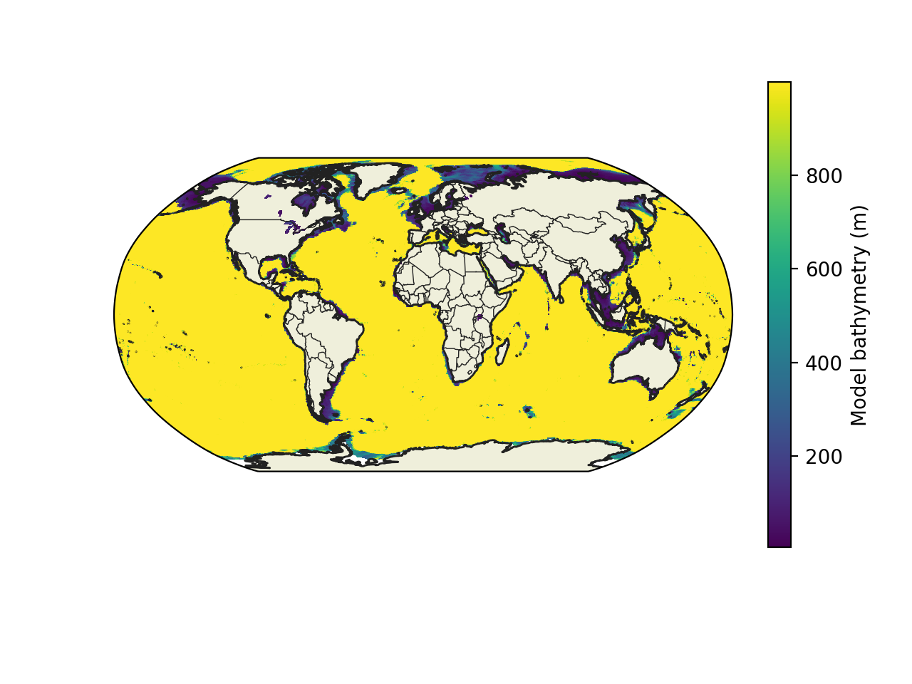
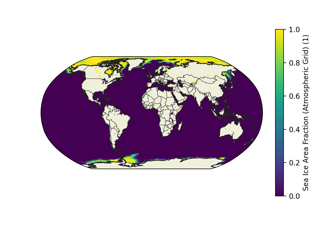
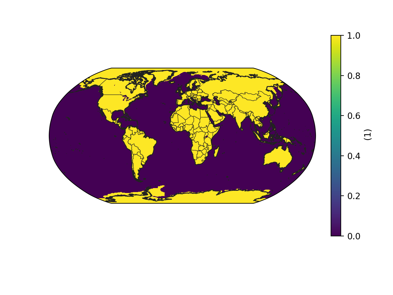
Fig 1: Model bathymetry Fig 2: Sea-ice cover Fig 3: Combined mask
Please note that sea-ice cover is only updated once daily.
- Values below the surface are there for convenience and simplicity: the fields would be more difficult to deal with if they contained voids. This can be problematic for many applications, such as time averages where the voids move around with time. However, extrapolating into the data voids can contaminate the "real" atmosphere. This happens if the parameter is archived in spectral space or if it's horizontally interpolated. The method for extrapolation below the surface is parameter dependent, but wind components and humidity are kept constant from the lowest model level, whereas temperature is linearly interpolated from the lowest model level to a surface temperature and then a cubic polynomial extrapolation is used thereafter.
Known issues
Currently, we are aware of these issues with ERA5:
- ERA5T: from 1 September to 13 December 2021, the final ERA5 product is different to ERA5T due to the correction of the assimilation of incorrect snow observations in central Asia. Although the differences are mostly limited to that region and mainly to surface parameters, in particular snow depth and soil moisture and to a lesser extent 2m temperature and 2m dewpoint temperature, all the resulting reanalysis fields can differ over the whole globe but should be within their range of uncertainty (which is estimated by the ensemble spread and which can be large for some parameters). On the CDS disks, the initial, ERA5T, fields have been overwritten (with the usual 2-3 month delay), i.e., for these months, access to the original CDS disk, ERA5T product is not possible after it has been overwritten. Potentially incorrect snow observations have been assimilated in ERA5 up to this time, when the effects became noticeable. The quality control of snow observations has been improved in ERA5 from September 2021 and from 15 November 2021 in ERA5T.
- ERA5 uncertainty: although small values of ensemble spread correctly mark more confident estimates than large values, numerical values are over confident. The spread does give an indication of the relative, random uncertainty in space and time.
- ERA5 suffers from an overly strong equatorial mesospheric jet, particularly in the transition seasons.
- From 2000 to 2006, ERA5 has a poor fit to radiosonde temperatures in the stratosphere, with a cold bias in the lower stratosphere. In addition, a warm bias higher up persists for much of the ERA5 period. The lower stratospheric cold bias was rectified in a re-run for the years 2000 to 2006, called ERA5.1, see "Resolved issues" below.
- Discontinuities in ERA5: The historic ERA5 data was produced by running several parallel experiments, each for a different period, which were then spliced together to create the final product. This can create discontinuities at the transition points.
- The analysed "2 metre temperature" can be larger than the forecast "Maximum temperature at 2 metres since previous post-processing".
- The analysed 10 metre wind speed (derived from the 10 metre wind components) can be larger than the forecast "10 metre wind gust since previous post-processing". This is because instantaneous winds in the CDS come from ERA5 analysis fields, while the gusts come from the short forecasts that connect analysis data assimilation windows.
- ERA5 diurnal cycle for near surface winds: the hourly data reveals a mismatch in the analysed near surface wind speed between the end of one assimilation cycle and the beginning of the next (which occurs at 9:00 - 10:00 and 21:00 - 22:00 UTC). This problem mostly occurs in low latitude oceanic regions, though it can also be seen over Europe and the USA. We cannot rectify this problem in the analyses. The forecast near surface winds show much better agreement between the assimilation cycles, at least on average, so if this mismatch is problematic for a particular application, our advice would be to use the forecast winds. The forecast near surface winds are available from MARS, see the section, Data organisation and how to download ERA5.
- ERA5 diurnal cycle for near surface temperature and humidity: some locations do suffer from a mismatch in the analysed values between the end of one assimilation cycle and the beginning of the next, in a similar fashion to that for the near surface winds (see above), but this problem is thought not to be so widespread as that for the near surface winds. The forecast values for near surface temperature and humidity are usually smoother than the analyses, but the forecast low level temperatures suffer from a cold bias over most parts of the globe. The forecast near surface temperature and humidity are available from MARS, see the section Data organisation and how to download ERA5.
- ERA5: large 10m winds: up to a few times per year, the analysed low level winds, eg 10m winds, become very large in a particular location, which varies amongst a few apparently preferred locations. The largest values seen so far are about 300 ms-1.
- ERA5 rain bombs: up to a few times per year, the rainfall (precipitation) can become extremely large in small areas. This problem occurs mostly over Africa, in regions of high orography.
- Large values of CAPE: occasionally, the Convective available potential energy in ERA5 is unrealistically large.
- Ship tracks in the SST: prior to September 2007, in the period when HadISST2 was used, ship tracks can be visible in the SST.
- Prior to 2014, the SST was not used over the Great Lakes to nudge the lake model. Consequently, the 2 metre temperature has an annual cycle that is too strong, with temperatures being too cold in winter and too warm in summer.
- The Potential Evaporation field (pev, parameter Id 228251) is largely underestimated over deserts and high-forested areas. This is due to a bug in the code that does not allow transpiration to occur in the situation where there is no low vegetation.
- Wave parameters (Table 7 above) for the three swell partitions: these parameters have been calculated incorrectly. The problem is most evident in the swell partition parameters involving the mean wave period: Mean wave period of first swell partition, Mean wave period of second swell partition and Mean wave period of third swell partition, where the periods are far too long.
- Surface photosynthetically available radiation (PAR) is too low in the version (CY41R2) of the ECMWF Integrated Forecasting System (IFS) used to produce ERA5, so PAR and clear sky PAR have not been published in ERA5. There is a bug in the calculation of PAR, with it being taken from the wrong parts of the spectrum. The shortwave bands include 0.442-0.625 micron, 0.625-0.778 micron and 0.778-1.24 micron. PAR should be coded to be the sum of the radiation in the first of these bands and 0.42 of the second (to account for the fact that PAR is normally defined to stop at 0.7 microns). However, in CY41R2, PAR is in fact calculated from the sum of the second band plus 0.42 of the third. We will try to fix this in a future cycle.
ERA5 forecast parameters are missing for the validity times of 1st January 1940 from 00 UTC to 06 UTC (except for forecast step=0). This problem occurs because the first forecast in ERA5 was initiated from 1st January 1940 at 06 UTC.
Maximum temperature at 2 metres since previous post-processing: in a small region over Peru, at 19 UTC, 2 August 2013, this forecast parameter exhibited erroneous values, which were greater than 50C. This occurrence is under investigation. Note, in general, we recommend that the hourly (analysed) "2 metre temperature" be used to construct the minimum and maximum over longer periods, such as a day.
- ERA5 sea-ice cover and 2 metre temperature: in the period 1979-1989, in a region just to the north of Greenland, the sea-ice cover outside of the melt season is too low and hence the 2 metre temperature is too high. For more information, see Section 3.5.4 of Low frequency variability and trends in surface air temperature and humidity from ERA5 and other datasets
- ERA5 sea-ice cover is missing in the Caspian Sea from late 2007 to 2013, inclusive.
- ERA5 sea-ice surface temperature (skin temperature) in the Arctic, during winter, can have a warm bias of 5K or more. This issue is most pronounced over thick snow-covered sea ice under cold clear-sky conditions, when the modelled conductive heat flux from the warm ocean underneath the ice and snow layer is too high. More information can be found in Batrak and Müller (2019) and Zampieri et al., (2023), the latter of which, also describes a method to improve on this bias.
- Altimeter wave height observations have not been available for ERA5 in the following periods (since coverage began in mid-1991): early February 2021 to mid-January 2022; mid-October 2023 onwards.
- ERA5 CDS: wind values are far too low on pressure levels at the poles in the CDS
- Snow present in Iberia throughout 1978 due to assimilation of erroneous in situ snow data. This has an effect on 2m temperature, which shows negative anomalies of several degrees Celsius. There is no snow present in ERA5-Land, as this snow data is not assimilated. However, the 2m temperature anomaly is present, as the forcing comes from the erroneous ERA5 data. These figures show ERA monthly averaged 2m temperature (t2m) and snow depth (sd) (38 to 43N, -8 to -6W), from 1940-2023, with 1978 highlighted in red. The same snow depth plot, limited to 1977-07 to 1979-04 shows more detail, with the period of erroneous snow depth in ERA5 extending from 1977-12 to 1979-03 in the monthly mean dataset.
From 24th to 29th June 2024 global SSTs in ERA5 remain constant, due to a technical error with delivery of the OSTIA SST product that is used. The data from 24th June 22:00 is persisted until new SSTs on 29th June 22:00. Changes in SST over the lakes can be seen during this period, as these are products of the lake model in ERA5. The plot shows mean SSTs 60S to 35N during this period, with this domain chosen to reduce the impact of changing SSTs in lakes.

Figure: Mean SST values 60S to 35N
From 11th to 18th September 2024 global sea ice concentration (SIC) in ERA5 remained constant, due to a technical error with delivery of the OSI-SAF product that is used. The data from 10th September 22:00 are persisted until 18th September 22:00. The plots show the mean SIC over the northern hemisphere (NH) and southern hemisphere (SH) during September 2024.


Figure: Mean SIC over the northern hemisphere (NH) and southern hemisphere (SH) during September 2024.
- Error in near-surface winds from the ERA5 reanalysis over the Southern Ocean near Antarctica. From May-October 1996 there is a semi-permanent cyclone which appears in ERA5 over the Amundsen Sea region (approximately 74 to 68°S, 206-260°E) which is highly unrealistic. This is due to the wrong station altitude sometimes being reported for the nearest observation station.
- Instabilities in CAPE close to the end of the 12-hourly assimilation window can lead to artifacts in the wind and temperature fields on pressure levels.
Resolved issues
ERA5.1 is a re-run of ERA5, for the years 2000 to 2006 only, and was produced to improve upon the cold bias in the lower stratosphere seen in ERA5.
- ERA5.1 CDS: If you retrieved ERA5.1 using the CDS API anytime before 20/05/2020 08:00 UTC, for any stream other than oper (i.e. streams: wave, enda, edmo, ewmo, edmm, ewmm, ewda, moda, wamd, mnth, wamo), you will need to request the data again. Prior to this date, stream oper would be delivered regardless of which stream was requested.
- ERA5 CDS: incorrect values of U/V on pressure levels in the CDS
- ERA5 CDS: Data corruption
- ERA5T rewritten: from 1 July to 17 November 2024, the final ERA5 product was different to ERA5T due to the correction of the assimilation of incorrect snow observations on the Alps. Although the differences were mostly limited to that region and mainly to surface parameters, in particular snow depth and soil moisture and to a lesser extent 2m temperature and 2m dewpoint temperature, all the resulting reanalysis fields can differ over the whole globe but should be within their range of uncertainty (which is estimated by the ensemble spread and which can be large for some parameters). On the CDS disks, the initial, ERA5T, fields have been overwritten (with the usual 2-3 month delay), i.e., for these months, access to the original CDS disk, ERA5T product is not possible after it has been overwritten. Potentially incorrect snow observations have been assimilated in ERA5 up to this time, when the effects became noticeable.
- ERA5T rewritten 1st - 6th January 2025: At the turn of 2025, an unfortunate technical issue with the production of ERA5 resulted in a large part of satellite observations not being used. This led to small but systematic differences, impacting mainly humidity in the tropics, and in lesser extent other ERA5 parameters as well from the 1st of January 2025 onwards. The issue was resolved and ERA5T and ERA5-Land-T were rewritten with the correct data from 12 UTC 1st January to 12 UTC 6th January 2025. The consolidated ERA5 and ERA5-Land will contain these corrected values.
User support
There is a range of user support available for ERA5, including a Knowledge Base (where this article resides), a Forum and a ticketed system for questions - for more information see the C3S Help and Support Page.
How to acknowledge and cite ERA5
If you have downloaded ERA5 data on the "CDS disks" and/or downloaded ERA5 data in MARS, using either the CDS API ('reanalysis-era5-complete' or'reanalysis-era5.1-complete') or via authorised direct access to MARS, please follow the instructions below:
In addition to the terms and conditions of the license(s), users must:
- cite the CDS catalogue entry;
- provide clear and visible attribution to the Copernicus programme and attribute each data product used;
Step 1: Check the licence for any attribution/reference clause
Step 2: Cite the CDS catalogue entry (as traceable source of data). Note that a catalogue entry for ERA5-complete and ERA5.1 is now also available in the CDS.
Step 3: Provide clear and visible attribution to the Copernicus programme and attribute each data product used (to accredit the creators of the data). Throughout the content of your publication, the dataset used is referred to as Author (YYYY)
The 3-steps procedure above is illustrated with this example: Use Case 2: ERA5 hourly data on single levels from 1940 to present
For complete details, please refer to How to acknowledge and cite a Climate Data Store (CDS) catalogue entry and the data published as part of it.
References
The ERA5 global reanalysis from 1940 to 2022
The ERA5 global reanalysis: Preliminary extension to 1950
Global stratospheric temperature bias and other stratospheric aspects of ERA5 and ERA5.1
Further ERA5 references are available from the ECMWF website.
